Chapter 11 SEM: Model Respecifications
In the prior two lessons we engaged in the first of two steps structural equation modeling. We first established the measurement model. Next we specified and evaluated a structural model, which included testing alternative models. In this lesson we consider how to use model statistics to consider respecifying the model through building and trimming. Further, we learn how to compare these models to determine if the fit is improved (i.e., a goal when we free parameters to be in relation with each other), stayed the same (i.e., a goal when we trim paths, thereby fixing their relation to 0.00), or deteriorated.
11.2 Respecifying Structural Models
There is general consensus ((Byrne, 2016b; Chou & Bentler, 2002)) that of the three types of approaches to model building (i.e., strictly confirmatory, alternative models, model generating (Joreskog, 1993)), that model generating is the most commonly used. This means that researchers will respecify the model by either adding paths or covariances, trimming paths or covariances, or both. At the risk of oversimplification, modelers generally take a model building or model trimming approaches. But of course – there is complexity and nuance that we should unravel.
11.2.1 Model Building
In model building, the researcher starts with a more parsimonious model and proceeds to a more general model. Chou and Bentler (2002) termed this forward searching. In general, this requires specifying a model that is overidentified (i.e., it has positive degrees of freedom). If the model does not fit the data well, we will request modification indices. These values are presented in the metric of the chi-square test and will tell us “by how much the chi-square value will decrease” if the two elements listed in each (of a long list) of the results is freed to relate (i.e., by a path or covariance). In a one-degree chi-square test, statistically significant change occurs when the modification index is greater than 3.841.
Freeing parameters is an activity that should be done with caution. Freeing a single parameter by adding a directional path or bidirectional covariance will reduce the degrees of freedom in the structural model by 1. Correspondingly, this respecified model will be the nesting model and will (in all likelihood) have better fit. The chi-square value will decrease by the amount indicated in the modification index and, presuming the parameter was freed because it would result in a statistically significant decrease in the unit of the chi-square, the respecified model with the additional path(s) may look as if it is a superior model. When fit is increasing incrementally, it can be tempting to keep freeing parameters until degrees of freedom are zero and the model is just identified. Doing so, risks overparameterization. This means that the model is overfit. Although it appears to fit the sample data well, it may fail to generalize to a different set of data that represents the population of interest. That is, the model is sample-specific which makes it less useful in making predictions or generalizing more broadly.
Thus, there are are cautions about model the forward searching approach:
- Any paths that are added (i.e., any parameters that are freed) should have strong theoretical justification.
- Any paths that are added should be statistically sensible. The procedure we use to produce modification indices, will produce them for every unsaturated paths. Sensible relations would generally include
- directional paths between variables in the structural model, and
- error covariances in the measurement model (for more on this see the lesson, CFA: Hierarchical and Nested Models
- Avoid adding paths that are not sensible. An example would be a path between an indicator in the measurement model and a structural variable.
- but do think about why the modification index might be suggesting such; perhaps it is a clue to an error.
11.2.2 Model Trimming
In model trimming, the researcher starts with a more general model or saturated (i.e., zero degrees of freedom in the structural model) and, on the basis of statistical criteria, trims non-significant (i.e., and low regression weight) paths from the model. Chou and Bentler (2002) termed this backward searching. The general process is to identify and delete non-essential paths one at a time and evaluate the “hit to the fit.” Given that the more saturated model is the nesting model, one can expect that trimmed, nested model will have fit that is incrementally lower. The hope is that the difference does not bring the global fit indices into thresholds that indicate poor fit and that, when compared statistically, the nested model is not statistically significantly different than the nesting model.
Several prominent researchers appear to favor the model trimming/backward searching approach. Chou and Bentler (2002) acknowledged that while the forward searching approach is commonly utilized its ability to find the true model has been questioned. Their Monte Carlo based test study demonstrated that a backward search approach that imposed constraints with the z and Wald(W) tests identified the true model with greater than 60% accuracy. Kenny’s (Kenny, 2012) SEM website and workshops have also advocated for a model trimming approach that generally starts with a just-identified (i.e., saturated, df = 0) model and trims paths, one-at-a-time, to see if the adequately fitting result resembled the theoretical model they identified, apriorily.
11.2.3 Restating Approaches to Respecification
The terms, concepts, and logic related to nesting, saturation, and respecification can be confusing. Hopefully, this table can help clarify their meaning and role.
| Approach to Respecification | Hypothesized (Original model) is | Comparison model(s) is | Typical Hope of \(\Delta\chi^2\) test |
|---|---|---|---|
| Model building, forward search | overidentified, df > 0 | more paths, fewer df | significant indicating additional path improved model fit |
| Model trimming, backward search | just-identified, df = 0 | fewer paths, more df | non-significant indicating deleted path did not lead to poorer model fit |
In today’s lesson, we will start with a rather complex, over-identified model. Following the example Byrne’s (Byrne, 2016a) chapter, we will first use modification indices to see about freeing parameters (i.e., adding paths) and then inspect nonsignificant paths for possible constraint (e.g., deletion).
11.3 Workflow for Evaluating a Structural Model
Below is the overall workflow for evaluating a structural model. Today our focus is the specification and evaluation of the structural model.
 Evaluating a structural model involves the following steps:
- A Priori Power Analysis
- Conduct an a priori power analysis to determine the appropriate sample size. _ Draw estimates of effect from pilot data and/or the literature.
- Scrubbing & Scoring
- Import data and format (i.e., variable naming, reverse-scoring) item level variables.
- Analyze item-level missingness.
- If using scales, create the mean scores of the scales.
- Determine and execute approach for managing missingness. Popular choices are available item analysis (e.g., Parent, 2013) and multiple imputation.
- Analyze scale-level missingness.
- Create a df with only the items (scaled in the proper direction).
- Data Diagnostics
- Evaluate univariate normality (i.e., one variable at a time) with Shapiro-Wilks tests; p < .05 indicates a violation of univariate normality.
- Evaluate multivariate normality (i.e., all continuously scaled variables simultaneously) with Mahalanobis test. Identify outliers (e.g., cases with Mahal values > 3 SDs from the centroid). Consider deleting (or transforming if there is an extreme-ish “jump” in the sorted values.
- Evaluate internal consistency of the scaled scores with Cronbach’s alpha or omega; the latter is increasingly preferred. Specify and evaluate a measurement model
- In this just-identified (saturated) model, all latent variables are specified as covarying.
- For LVs with 3 items or more, remember to set a marker/reference variable,
- For LVs with 2 items, constrain the loadings to be equal,
- For single-item indicators fix the error variance to zero (or a non-zero estimate of unreliability).
- Evaluate results with global (e.g., X2, CFI, RMSEA, SRMR) and local (i.e., factor loadings and covariances) fit indices.
- In the event of poor fit, respecify LVs with multiple indicators with parcels.
- Nested alternative measurement models can be compared with Χ2 difference, ΔCFI tests; non-nested models with AIC, and BIC tests .
- Specify and evaluate a structural model.
- Replace the covariances with paths that represent the a priori hypotheses.
- These models could take a variety of forms.
- It is possible to respecify models through trimming or building approaches.
- Evaluate results using
- global fit indices (e.g., X2, CFI, RMSEA, SRMS),
- local fit indices (i.e., strength and significance of factor loadings, covariances, and additional model parameters [e.g., indirect effects]).
- Consider respecifying and evaluating one or more alternative models.
- Forward searching involves freeing parameters (adding paths or covariances) and can use modification indices as a guide.
- Backward searching involves restraining parameters (deleting paths or covariances) and can use low and non-significant paths as a guide.
- Compare the fit of the alternate models.
- Nested models can be compared with Χ2 difference and ΔCFI tests.
- Non-nested models can be compared with AIC and BIC (lower values suggest better fit).
- Replace the covariances with paths that represent the a priori hypotheses.
- Quick Guide for Global and Comparative Fit Statistics.
- \(\chi^2\), p < .05; this test is sensitive to sample size and this value can be difficult to attain
- CFI > .95 (or at least .90)
- RMSEA (and associated 90%CI) are < .05 ( < .08, or at least < .10)
- SRMR < .08 (or at least <.10)
- Combination rule: CFI < .95 and SRMR < .08
- AIC and BIC are compared; the lowest values suggest better models
- \(\chi^2\Delta\) is statistically significant; the model with the superior fit is the better model
- \(\delta CFI\) is greater than 0.01; the model with CFI values closest to 1.0 has better fit
11.4 Research Vignette
Once again the research vignette comes from the Lewis, Williams, Peppers, and Gadson’s (2017) study titled, “Applying Intersectionality to Explore the Relations Between Gendered Racism and Health Among Black Women.” The study was published in the Journal of Counseling Psychology. Participants were 231 Black women who completed an online survey.
Variables used in the study included:
GRMS: Gendered Racial Microaggressions Scale (J. A. Lewis & Neville, 2015) is a 26-item scale that assesses the frequency of nonverbal, verbal, and behavioral negative racial and gender slights experienced by Black women. Scaling is along six points ranging from 0 (never) to 5 (once a week or more). Higher scores indicate a greater frequency of gendered racial microaggressions. An example item is, “Someone has made a sexually inappropriate comment about my butt, hips, or thighs.”
MntlHlth and PhysHlth: Short Form Health Survey - Version 2 (Ware et al., 1995) is a 12-item scale used to report self-reported mental (six items) and physical health (six items). Higher scores indicate higher mental health (e.g., little or no psychological ldistress) and physical health (e.g., little or no reported symptoms in physical functioning). An example of an item assessing mental health was, “How much of the time during the last 4 weeks have you felt calm and peaceful?”; an example of a physical health item was, “During the past 4 weeks, how much did pain interfere with your normal work?”
Sprtlty, SocSup, Engmgt, and DisEngmt are four subscales from the Brief Coping with Problems Experienced Inventory (Carver, 1997). The 28 items on this scale are presented on a 4-point scale ranging from 1 (I usually do not do this at all) to 4(I usually do this a lot). Higher scores indicate a respondents’ tendency to engage in a particular strategy. Instructions were modified to ask how the female participants responded to recent experiences of racism and sexism as Black women. The four subscales included spirituality (religion, acceptance, planning), interconnectedness/social support (vent emotions, emotional support,instrumental social support), problem-oriented/engagement coping (active coping, humor, positive reinterpretation/positive reframing), and disengagement coping (behavioral disengagement, substance abuse, denial, self-blame, self-distraction).
GRIcntlty: The Multidimensional Inventory of Black Identity Centrality subscale (Sellers et al., n.d.) was modified to measure the intersection of racial and gender identity centrality. The scale included 10 items scaled from 1 (strongly disagree) to 7 (strongly agree). An example item was, “Being a Black woman is important to my self-image.” Higher scores indicated higher levels of gendered racial identity centrality.
Today we will use the simulated data to evaluate a model that was suggested by a figure in the journal (one IV, four mediators, two dependent variables) but was not tested as a single structural model. Rather, the authors ran a series of four simple mediations per dependent variable for a total of eight separate analyses. The authors do not elaborate on their rationale for this appraoch. My guess is that they were limited in design by their use of ordinary least squares with the PROCESS macro in SPSS. Additionally, they may have been concerned about power when they considered a more complicated, latent variable, design.
Specifically, we will specify a parallel mediation model where two dependent variables (i.e., mental health, physical health) are predicted directly from gendered racial microaggressions and indirectly through four coping strategies (i.e., spirituality, social support, engagement, disengagement).
11.4.1 Simulating the data from the journal article
The lavaan::simulateData function was used. If you have taken psychometrics, you may recognize the code as one that creates latent variables form item-level data. In trying to be as authentic as possible, we retrieved factor loadings from psychometrically oriented articles that evaluated the measures (Nadal, 2011; Veit & Ware, 1983). For all others we specified a factor loading of 0.80. We then approximated the measurement model by specifying the correlations between the latent variable. We sourced these from the correlation matrix from the research vignette (J. A. Lewis et al., 2017). The process created data with multiple decimals and values that exceeded the boundaries of the variables. For example, in all scales there were negative values. Therefore, the final element of the simulation was a linear transformation that rescaled the variables back to the range described in the journal article and rounding the values to integer (i.e., with no decimal places).
#Entering the intercorrelations, means, and standard deviations from the journal article


Lewis_generating_model <- '
        #measurement model
        GRMS  =~ .69*Ob1 + .69*Ob2 + .60*Ob3 + .59*Ob4 + .55*Ob5 + .55*Ob6 + .54*Ob7 + .50*Ob8 + .41*Ob9 + .41*Ob10 + .93*Ma1 + .81*Ma2 + .69*Ma3 + .67*Ma4 + .61*Ma5 + .58*Ma6 + .54*Ma7 + .59*St1 + .55*St2 + .54*St3 + .54*St4 + .51*St5 + .70*An1 + .69*An2 + .68*An3
        MntlHlth  =~ .8*MH1 + .8*MH2 + .8*MH3 + .8*MH4 + .8*MH5 + .8*MH6
        PhysHlth  =~ .8*PhH1 + .8*PhH2 + .8*PhH3 + .8*PhH4 + .8*PhH5 + .8*PhH6
        Spirituality  =~ .8*Spirit1 + .8*Spirit2
        SocSupport  =~ .8*SocS1 + .8*SocS2
        Engagement  =~ .8*Eng1 + .8*Eng2
        Disengagement  =~  .8*dEng1 + .8*dEng2
        GRIC  =~ .8*Cntrlty1 + .8*Cntrlty2 + .8*Cntrlty3 + .8*Cntrlty4 + .8*Cntrlty5 + .8*Cntrlty6 + .8*Cntrlty7 + .8*Cntrlty8 + .8*Cntrlty9 + .8*Cntrlty10

        #Means
         GRMS ~ 1.99*1
         Spirituality ~2.82*1
         SocSupport ~ 2.48*1
         Engagement ~ 2.32*1
         Disengagement ~ 1.75*1
         GRIC ~ 5.71*1
         MntlHlth ~3.56*1 #Lewis et al used sums instead of means, I recast as means to facilitate simulation
         PhysHlth ~ 3.51*1 #Lewis et al used sums instead of means, I recast as means to facilitate simulation

        #Correlations
         GRMS ~ 0.20*Spirituality
         GRMS ~ 0.28*SocSupport
         GRMS ~ 0.30*Engagement
         GRMS ~ 0.41*Disengagement
         GRMS ~ 0.19*GRIC
         GRMS ~ -0.32*MntlHlth
         GRMS ~ -0.18*PhysHlth

         Spirituality ~ 0.49*SocSupport
         Spirituality ~ 0.57*Engagement
         Spirituality ~ 0.22*Disengagement
         Spirituality ~ 0.12*GRIC
         Spirituality ~ -0.06*MntlHlth
         Spirituality ~ -0.13*PhysHlth

         SocSupport ~ 0.46*Engagement
         SocSupport ~ 0.26*Disengagement
         SocSupport ~ 0.38*GRIC
         SocSupport ~ -0.18*MntlHlth
         SocSupport ~ -0.08*PhysHlth

         Engagement ~ 0.37*Disengagement
         Engagement ~ 0.08*GRIC
         Engagement ~ -0.14*MntlHlth
         Engagement ~ -0.06*PhysHlth

         Disengagement ~ 0.05*GRIC
         Disengagement ~ -0.54*MntlHlth
         Disengagement ~ -0.28*PhysHlth

         GRIC ~ -0.10*MntlHlth
         GRIC ~ 0.14*PhysHlth

         MntlHlth ~ 0.47*PhysHlth
        '

set.seed(230925)
dfLewis <- lavaan::simulateData(model = Lewis_generating_model,
                              model.type = "sem",
                              meanstructure = T,
                              sample.nobs=231,
                              standardized=FALSE)

#used to retrieve column indices used in the rescaling script below
#col_index <- as.data.frame(colnames(dfLewis))

for(i in 1:ncol(dfLewis)){  # for loop to go through each column of the dataframe
  if(i >= 1 & i <= 25){   # apply only to GRMS variables
    dfLewis[,i] <- scales::rescale(dfLewis[,i], c(0, 5))
  }
  if(i >= 26 & i <= 37){   # apply only to mental and physical health variables
    dfLewis[,i] <- scales::rescale(dfLewis[,i], c(0, 6))
  }
  if(i >= 38 & i <= 45){   # apply only to coping variables
    dfLewis[,i] <- scales::rescale(dfLewis[,i], c(1, 4))
  }
  if(i >= 46 & i <= 55){   # apply only to GRIC variables
    dfLewis[,i] <- scales::rescale(dfLewis[,i], c(1, 7))
  }
}

#rounding to integers so that the data resembles that which was collected
library(tidyverse)
dfLewis <- dfLewis %>% round(0)

#quick check of my work
#psych::describe(dfLewis)
The script below allows you to store the simulated data as a file on your computer. This is optional – the entire lesson can be worked with the simulated data.
If you prefer the .rds format, use this script (remove the hashtags). The .rds format has the advantage of preserving any formatting of variables. A disadvantage is that you cannot open these files outside of the R environment.
Script to save the data to your computer as an .rds file.
Once saved, you could clean your environment and bring the data back in from its .csv format.
If you prefer the .csv format (think “Excel lite”) use this script (remove the hashtags). An advantage of the .csv format is that you can open the data outside of the R environment. A disadvantage is that it may not retain any formatting of variables
Script to save the data to your computer as a .csv file.
Once saved, you could clean your environment and bring the data back in from its .csv format.
11.5 Scrubbing, Scoring, and Data Diagnostics
Because the focus of this lesson is on the specific topic of specifying and evaluating a structural model for SEM and have used simulated data, we are skipping many of the steps in scrubbing, scoring and data diagnostics. If this were real, raw, data, it would be important to scrub, if needed score, and conduct data diagnostics to evaluate the suitability of the data for the proposes analyses.
11.6 Script for Specifying Models in lavaan
SEM in lavaan requires fluency with the R script. Below is a brief overview of the operators we use most frequently:
- Latent variables (factors) must be defined by their manifest or latent indicators.
- the special operator (=~, is measured/defined by) is used for this
- Example: f1 =~ y1 + y2 + y3
- Regression equations use the single tilda (~, is regressed on)
- place DV (y) on left of operator
- place IVs, separate by + on the right
- Example: y ~ f1 + f2 + x1 + x2
- f is a latent variable in this example
- y, x1, and x2 are observed variables in this example
- An asterisk can affix a label in subsequent calculations and in interpreting output
- Variances and covariances are specified with a double tilde operator (~~, is correlated with)
- Example of variance: y1 ~~ y1 (the relationship with itself)
- Example of covariance: y1 ~~ y2 (relationship with another variable)
- Example of covariance of a factor: f1 ~~ f2 *Intercepts (~ 1) for observed and LVs are simple, intercept-only regression formulas
- Example of variable intercept: y1 ~ 1
- Example of factor intercept: f1 ~ 1
A complete lavaan model is a combination of these formula types, enclosed between single quotation models. Readibility of model syntax is improved by:
- splitting formulas over multiple lines
- using blank lines within single quote
- labeling with the hashtag
11.7 Quick Specification of the Measurement Model
Recall that the first step in establishing a structural model is to specify, evaluate, and if necessary re-specify the measurement model. For this data I have specified the measurement model as follows:
- Gendered Racial Microaggressions Scale (GRMS): randomly assign the 26 items to 3 parcels.
- Mental health (MH): randomly assign the 6 items to 3 parcels.
- Physical health (PhH): randomly assign the 6 items to 3 parcels.
- Coping strategies (spiritual/Spr, social support (SSp), engagement (Eng), disengagement (dEng): Constrain the loadings for each of the two variables per construct to be equal.
For more information on establishing measurement models please visit the lesson on establishing the measurement model. Here is a representation of the measurement model we are specifying.
 To proceed with this approach, I first need to create parcels for the GRMS, MH, and PhH scales. This code randomly assigns the GRMS items to three parcels.
set.seed(230916)
items <- c("Ob1", "Ob2", "Ob3", "Ob4", "Ob5", "Ob6", "Ob7", "Ob8", "Ob9",
    "Ob10", "Ma1", "Ma2", "Ma3", "Ma4", "Ma5", "Ma6", "Ma7", "St1", "St2",
    "St3", "St4", "St5", "An1", "An2")
parcels <- c("GRMS_p1", "GRMS_p_2", "GRMS_p3")
data.frame(items = sample(items), parcel = rep(parcels, length = length(items)))
## items parcel
## 1 Ma3 GRMS_p1
## 2 Ob7 GRMS_p_2
## 3 Ob9 GRMS_p3
## 4 Ma7 GRMS_p1
## 5 Ma5 GRMS_p_2
## 6 Ob2 GRMS_p3
## 7 Ma1 GRMS_p1
## 8 An1 GRMS_p_2
## 9 Ob4 GRMS_p3
## 10 Ob1 GRMS_p1
## 11 St3 GRMS_p_2
## 12 Ob6 GRMS_p3
## 13 St2 GRMS_p1
## 14 Ob5 GRMS_p_2
## 15 Ob10 GRMS_p3
## 16 Ob8 GRMS_p1
## 17 Ma6 GRMS_p_2
## 18 St5 GRMS_p3
## 19 An2 GRMS_p1
## 20 Ma2 GRMS_p_2
## 21 Ob3 GRMS_p3
## 22 Ma4 GRMS_p1
## 23 St1 GRMS_p_2
## 24 St4 GRMS_p3We can now create the parcels using the same scoring procedure as we did for the REMS and CMI instruments.
GRMS_p1_vars <- c("Ma3", "Ma7", "Ma1", "Ob1", "St2", "Ob8", "An2", "Ma4")
GRMS_p2_vars <- c("Ob7", "Ma5", "An1", "St3", "Ob5", "Ma6", "Ma2", "St1")
GRMS_p3_vars <- c("Ob9", "Ob2", "Ob4", "Ob6", "Ob10", "St5", "Ob3", "St4")

dfLewis$p1GRMS <- sjstats::mean_n(dfLewis[, GRMS_p1_vars], 0.75)
dfLewis$p2GRMS <- sjstats::mean_n(dfLewis[, GRMS_p2_vars], 0.75)
dfLewis$p3GRMS <- sjstats::mean_n(dfLewis[, GRMS_p3_vars], 0.75)

# If the scoring code above does not work for you, try the format
# below which involves inserting to periods in front of the variable
# list. One example is provided. dfLewis$p3PWB <-
# sjstats::mean_n(dfLewis[, ..PWB_p3_vars], .75)
This code randomly assigns the mental health items to three parcels.
set.seed(230916)
items <- c("MH1", "MH2", "MH3", "MH4", "MH5", "MH6")
parcels <- c("MH_p1", "MH_p2", "MH_p3")
data.frame(items = sample(items), parcel = rep(parcels, length = length(items)))
## items parcel
## 1 MH5 MH_p1
## 2 MH1 MH_p2
## 3 MH4 MH_p3
## 4 MH6 MH_p1
## 5 MH3 MH_p2
## 6 MH2 MH_p3This code provides means for each of the three REMS parcels.
MH_p1_vars <- c("MH5", "MH6")
MH_p2_vars <- c("MH1", "MH3")
MH_p3_vars <- c("MH4", "MH2")

dfLewis$p1MH <- sjstats::mean_n(dfLewis[, MH_p1_vars], 0.75)
dfLewis$p2MH <- sjstats::mean_n(dfLewis[, MH_p2_vars], 0.75)
dfLewis$p3MH <- sjstats::mean_n(dfLewis[, MH_p3_vars], 0.75)

# If the scoring code above does not work for you, try the format
# below which involves inserting to periods in front of the variable
# list. One example is provided. dfLewis$p3REMS <-
# sjstats::mean_n(dfLewis[, ..REMS_p3_vars], .80)
This code randomly assigns the physical health items to three parcels.
set.seed(230916)
items <- c("PhH1", "PhH2", "PhH3", "PhH4", "PhH5", "PhH6")
parcels <- c("PhH_p1", "PhH_p2", "PhH_p3")
data.frame(items = sample(items), parcel = rep(parcels, length = length(items)))
## items parcel
## 1 PhH5 PhH_p1
## 2 PhH1 PhH_p2
## 3 PhH4 PhH_p3
## 4 PhH6 PhH_p1
## 5 PhH3 PhH_p2
## 6 PhH2 PhH_p3This code provides means for each of the three REMS parcels.
PhH_p1_vars <- c("PhH5", "PhH6")
PhH_p2_vars <- c("PhH1", "PhH3")
PhH_p3_vars <- c("PhH4", "PhH2")

dfLewis$p1PhH <- sjstats::mean_n(dfLewis[, PhH_p1_vars], 0.75)
dfLewis$p2PhH <- sjstats::mean_n(dfLewis[, PhH_p2_vars], 0.75)
dfLewis$p3PhH <- sjstats::mean_n(dfLewis[, PhH_p3_vars], 0.75)

# If the scoring code above does not work for you, try the format
# below which involves inserting to periods in front of the variable
# list. One example is provided. dfLewis$p3REMS <-
# sjstats::mean_n(dfLewis[, ..REMS_p3_vars], .80)
Below is code for specifying the measurement model. Each of the latent variables/factors (REMS, CMI, PWB) is identified by three parcels. Each of the latent variables is allowed to covary with the others.
msmt_mod <- "
        ##measurement model
         GRMS =~ p1GRMS + p2GRMS + p3GRMS
         MH =~ p1MH + p2MH + p3MH
         PhH =~ p1PhH + p2PhH + p3PhH
         Spr =~ v1*Spirit1 + v1*Spirit2
         SSp =~ v2*SocS1 + v2*SocS2
         Eng =~ v3*Eng1 + v3*Eng2
         dEng =~ v4*dEng1 + v4*dEng2


        # Covariances
         GRMS ~~ MH
         GRMS ~~ PhH
         GRMS ~~ Spr
         GRMS ~~ SSp
         GRMS ~~ Eng
         GRMS ~~ dEng
         MH ~~ PhH
         MH ~~ Spr
         MH ~~ SSp
         MH ~~ Eng
         MH ~~ dEng
         PhH ~~ Spr
         PhH ~~ SSp
         PhH ~~ Eng
         PhH ~~ dEng
         Spr  ~~ SSp
         Spr  ~~ Eng
         Spr  ~~ dEng
         SSp ~~ Eng
         SSp ~~ dEng
         Eng ~~ dEng

        "

set.seed(230916)
msmt_fit <- lavaan::cfa(msmt_mod, data = dfLewis, missing = "fiml")
msmt_fit_sum <- lavaan::summary(msmt_fit, fit.measures = TRUE, standardized = TRUE)
msmt_fit_pEsts <- lavaan::parameterEstimates(msmt_fit, boot.ci.type = "bca.simple",
    standardized = TRUE)
msmt_fit_sum
## lavaan 0.6.17 ended normally after 106 iterations
##
## Estimator ML
## Optimization method NLMINB
## Number of model parameters 68
##
## Number of observations 231
## Number of missing patterns 1
##
## Model Test User Model:
##
## Test statistic 94.122
## Degrees of freedom 102
## P-value (Chi-square) 0.698
##
## Model Test Baseline Model:
##
## Test statistic 2104.157
## Degrees of freedom 136
## P-value 0.000
##
## User Model versus Baseline Model:
##
## Comparative Fit Index (CFI) 1.000
## Tucker-Lewis Index (TLI) 1.005
##
## Robust Comparative Fit Index (CFI) 1.000
## Robust Tucker-Lewis Index (TLI) 1.005
##
## Loglikelihood and Information Criteria:
##
## Loglikelihood user model (H0) -3376.747
## Loglikelihood unrestricted model (H1) -3329.686
##
## Akaike (AIC) 6889.494
## Bayesian (BIC) 7123.579
## Sample-size adjusted Bayesian (SABIC) 6908.057
##
## Root Mean Square Error of Approximation:
##
## RMSEA 0.000
## 90 Percent confidence interval - lower 0.000
## 90 Percent confidence interval - upper 0.028
## P-value H_0: RMSEA <= 0.050 1.000
## P-value H_0: RMSEA >= 0.080 0.000
##
## Robust RMSEA 0.000
## 90 Percent confidence interval - lower 0.000
## 90 Percent confidence interval - upper 0.028
## P-value H_0: Robust RMSEA <= 0.050 1.000
## P-value H_0: Robust RMSEA >= 0.080 0.000
##
## Standardized Root Mean Square Residual:
##
## SRMR 0.034
##
## Parameter Estimates:
##
## Standard errors Standard
## Information Observed
## Observed information based on Hessian
##
## Latent Variables:
## Estimate Std.Err z-value P(>|z|) Std.lv Std.all
## GRMS =~
## p1GRMS 1.000 0.726 0.956
## p2GRMS 1.014 0.030 34.037 0.000 0.736 0.961
## p3GRMS 0.904 0.030 30.069 0.000 0.656 0.934
## MH =~
## p1MH 1.000 0.624 0.765
## p2MH 1.237 0.128 9.696 0.000 0.773 0.728
## p3MH 1.241 0.112 11.044 0.000 0.775 0.776
## PhH =~
## p1PhH 1.000 0.600 0.662
## p2PhH 0.997 0.125 7.959 0.000 0.598 0.714
## p3PhH 1.060 0.139 7.643 0.000 0.636 0.727
## Spr =~
## Spirit1 (v1) 1.000 0.488 0.730
## Spirit2 (v1) 1.000 0.488 0.762
## SSp =~
## SocS1 (v2) 1.000 0.425 0.704
## SocS2 (v2) 1.000 0.425 0.654
## Eng =~
## Eng1 (v3) 1.000 0.409 0.612
## Eng2 (v3) 1.000 0.409 0.701
## dEng =~
## dEng1 (v4) 1.000 0.410 0.684
## dEng2 (v4) 1.000 0.410 0.652
##
## Covariances:
## Estimate Std.Err z-value P(>|z|) Std.lv Std.all
## GRMS ~~
## MH -0.290 0.042 -6.868 0.000 -0.639 -0.639
## PhH -0.185 0.039 -4.698 0.000 -0.425 -0.425
## Spr 0.289 0.034 8.445 0.000 0.815 0.815
## SSp 0.212 0.030 7.160 0.000 0.689 0.689
## Eng 0.204 0.029 7.054 0.000 0.689 0.689
## dEng 0.202 0.029 7.008 0.000 0.680 0.680
## MH ~~
## PhH 0.200 0.040 5.041 0.000 0.533 0.533
## Spr -0.155 0.030 -5.177 0.000 -0.507 -0.507
## SSp -0.113 0.027 -4.222 0.000 -0.427 -0.427
## Eng -0.090 0.025 -3.558 0.000 -0.353 -0.353
## dEng -0.168 0.028 -6.022 0.000 -0.656 -0.656
## PhH ~~
## Spr -0.090 0.028 -3.205 0.001 -0.307 -0.307
## SSp -0.069 0.026 -2.699 0.007 -0.271 -0.271
## Eng -0.052 0.025 -2.111 0.035 -0.212 -0.212
## dEng -0.101 0.026 -3.830 0.000 -0.411 -0.411
## Spr ~~
## SSp 0.153 0.023 6.739 0.000 0.738 0.738
## Eng 0.140 0.022 6.409 0.000 0.704 0.704
## dEng 0.129 0.022 5.998 0.000 0.646 0.646
## SSp ~~
## Eng 0.076 0.019 4.005 0.000 0.439 0.439
## dEng 0.070 0.019 3.693 0.000 0.400 0.400
## Eng ~~
## dEng 0.088 0.019 4.657 0.000 0.525 0.525
##
## Intercepts:
## Estimate Std.Err z-value P(>|z|) Std.lv Std.all
## .p1GRMS 2.592 0.050 51.897 0.000 2.592 3.415
## .p2GRMS 2.545 0.050 50.567 0.000 2.545 3.327
## .p3GRMS 2.579 0.046 55.829 0.000 2.579 3.673
## .p1MH 3.582 0.054 66.695 0.000 3.582 4.388
## .p2MH 2.866 0.070 41.068 0.000 2.866 2.702
## .p3MH 3.035 0.066 46.200 0.000 3.035 3.040
## .p1PhH 3.128 0.060 52.418 0.000 3.128 3.449
## .p2PhH 2.652 0.055 48.093 0.000 2.652 3.164
## .p3PhH 3.067 0.058 53.298 0.000 3.067 3.507
## .Spirit1 2.511 0.044 57.110 0.000 2.511 3.758
## .Spirit2 2.437 0.042 57.882 0.000 2.437 3.808
## .SocS1 2.550 0.040 64.254 0.000 2.550 4.228
## .SocS2 2.758 0.043 64.576 0.000 2.758 4.249
## .Eng1 2.437 0.044 55.427 0.000 2.437 3.647
## .Eng2 2.515 0.038 65.479 0.000 2.515 4.308
## .dEng1 2.502 0.039 63.518 0.000 2.502 4.179
## .dEng2 2.455 0.041 59.357 0.000 2.455 3.905
##
## Variances:
## Estimate Std.Err z-value P(>|z|) Std.lv Std.all
## .p1GRMS 0.050 0.008 6.600 0.000 0.050 0.086
## .p2GRMS 0.044 0.007 6.015 0.000 0.044 0.076
## .p3GRMS 0.063 0.008 8.289 0.000 0.063 0.128
## .p1MH 0.277 0.037 7.437 0.000 0.277 0.415
## .p2MH 0.528 0.067 7.935 0.000 0.528 0.469
## .p3MH 0.396 0.055 7.225 0.000 0.396 0.397
## .p1PhH 0.463 0.058 7.996 0.000 0.463 0.562
## .p2PhH 0.344 0.049 7.098 0.000 0.344 0.490
## .p3PhH 0.360 0.054 6.723 0.000 0.360 0.471
## .Spirit1 0.208 0.026 8.152 0.000 0.208 0.467
## .Spirit2 0.171 0.023 7.433 0.000 0.171 0.419
## .SocS1 0.183 0.025 7.225 0.000 0.183 0.504
## .SocS2 0.241 0.029 8.235 0.000 0.241 0.572
## .Eng1 0.279 0.032 8.627 0.000 0.279 0.625
## .Eng2 0.173 0.025 6.893 0.000 0.173 0.509
## .dEng1 0.191 0.025 7.482 0.000 0.191 0.532
## .dEng2 0.227 0.028 8.127 0.000 0.227 0.575
## GRMS 0.527 0.054 9.796 0.000 1.000 1.000
## MH 0.390 0.062 6.241 0.000 1.000 1.000
## PhH 0.360 0.074 4.854 0.000 1.000 1.000
## Spr 0.238 0.032 7.412 0.000 1.000 1.000
## SSp 0.180 0.028 6.378 0.000 1.000 1.000
## Eng 0.167 0.028 6.042 0.000 1.000 1.000
## dEng 0.168 0.027 6.208 0.000 1.000 1.000# msmt_fit_pEsts #although creating the object is useful to export as
# a .csv I didn't ask it to print into the bookThe factor loadings were all strong, statistically significant, and properly valenced. Further, global fit statistics were within acceptable thresholds (\(\chi^2(102) = 94.122, p = 0.698, CFI = 1.000, RMSEA = 0.000, 90CI[0.000, 0.028], SRMR = 0.034\)).
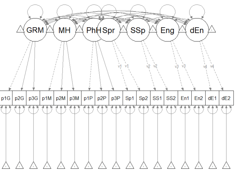
The figure below is an illustration of our measurement model with its results. It also conveys that each latent variable is indicated by three parcels and all of the latent variables are allowed to covary.
semPlot::semPaths(msmt_fit, what = "col", whatLabels = "stand", sizeMan = 5,
    node.width = 1, edge.label.cex = 0.75, style = "lisrel", mar = c(5,
        5, 5, 5))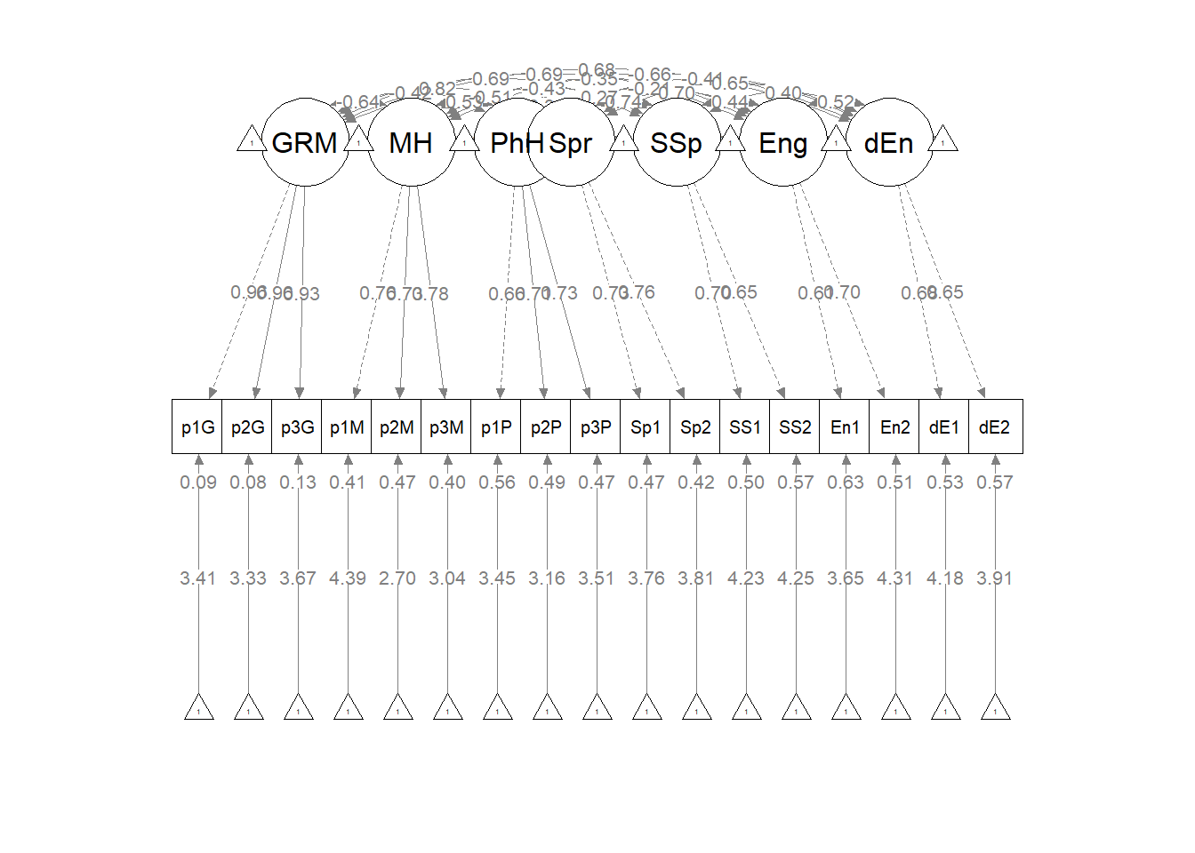
# semPlot::semPaths(msmt_fit) #ignore -- used to create a no-results
# figure earlier in the chapter
Below is script that will export the global fit indices (via tidySEM::table_fit) and the parameter estimates (e.g., factor loadings, structural regression weights, and parameters we requested such as the indirect effect) to .csv files that you can manipulate outside of R.
## Registered S3 method overwritten by 'tidySEM':
##   method          from
## predict.MxModel OpenMxwrite.csv(msmt_fitstats, file = "msmt_fitstats.csv")
# the code below writes the parameter estimates into a .csv file
write.csv(msmt_fit_pEsts, file = "msmt_pEsts.csv")Here’s how I might write an APA style summary of establishing the measurement model.
Analyzing our proposed multiple mediator model followed the two-step procedure of first evaluating a measurement model with acceptable fit to the data and then proceeding to test the structural model. Given that different researchers recommend somewhat differing thresholds to determine the adequacy of fit, We used the following as evidence of good fit: comparative fit indix (CFI) \(\geq 0.95\), root-mean-square error of approximation (RMSEA) \(\leq 0.06\), and the standard root-mean-square residual (SRMR) \(\leq 0.08\). To establish aceptable fit, we used CFI \(\geq 0.90\), RMSEA \(\leq 0.10\), and SRMR \(\leq 0.10\) (Weston & Gore, 2006).
To evaluate the measurement model we followed recommendations by Little et al. (T. D. Little et al., 2002, 2013). Specifically, each latent variable with six or more indicators was represented by three parcels. Parcels were created by randomly assigning scale items to the parcels and then calculating the mean, if at least 65% of the items were non-missing. For the four latent variables with only two indicators each, we constrained the factor loadings to be equal. Factor loadings were all strong, statistically significant, and properly valenced. Global fit statistics were within acceptable thresholds (\(\chi^2(102) = 94.122, p = 0.698, CFI = 1.000, RMSEA = 0.000, 90CI[0.000, 0.028], SRMR = 0.034\)). Thus, we proceeded to testing the structural model.
Table 1
| Factor Loadings for the Measurement Model |
|---|
| Latent variable and indicator | est | SE | p | est_std |
| Gendered Racial Microaggressions | ||||
| Parcel 1 | 1.000 | 0.000 | 0.956 | |
| Parcel 2 | 1.014 | 0.030 | <0.001 | 0.961 |
| Parcel 3 | 1.904 | 0.030 | <0.001 | 0.934 |
| Mental Health | ||||
| Parcel 1 | 1.000 | 0.000 | 0.765 | |
| Parcel 2 | 1.237 | 0.128 | <0.001 | 0.728 |
| Parcel 3 | 1.241 | 0.112 | <0.001 | 0.776 |
| Physical Health | ||||
| Parcel 1 | 1.000 | 0.000 | 0.662 | |
| Parcel 2 | 0.997 | 0.125 | <0.001 | 0.714 |
| Parcel 3 | 1.060 | 0.139 | <0.001 | 0.727 |
| Spiritual Coping | ||||
| Item 1 | 1.000 | 0.000 | 0.730 | |
| Item 2 | 1.000 | 0.000 | 0.762 | |
| Social Support Coping | ||||
| Item 1 | 1.000 | 0.000 | 0.704 | |
| Item 2 | 1.000 | 0.000 | 0.654 | |
| Engagement Coping | ||||
| Item 1 | 1.000 | 0.000 | 0.612 | |
| Item 2 | 1.000 | 0.000 | 0.701 | |
| Disengagement Coping | ||||
| Item 1 | 1.000 | 0.000 | 0.684 | |
| Item 2 | 1.000 | 0.000 | 0.652 |
Having established that our measurement model is adequate, we are ready to replace the covariances between latent variables with the paths (directional) and covariances (bidirectional) we hypothesize. These paths and covariances are soft hypotheses. That is, we are “freeing” them to relate. In SEM, hard hypotheses are where no path/covariance exists and the relationship between these variables is “fixed” to zero. This is directly related to degrees of freedom and the identification status (just-identified, over-identified, underidentified) of the model.
11.8 Specifying and Evaluating the Hypothesized Structural Model
As described more completely in the lesson on specifying and evaluating the structural model, the structural model evaluates the hypothesized relations between the latent variables. The structural model is typically more parsimonious (i.e., not saturated) than the measurement model and is characterized by directional paths (not covariances) between some (not all) of the variables.
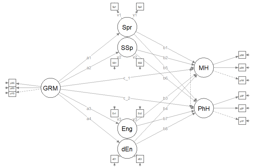
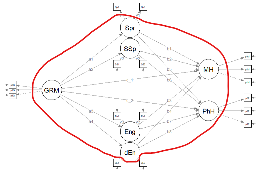
Here’s a quick reminder of the hypothesized model we are testing. Using data simulated from the Lewis et al. (2017)article, we are evaluating a parallel mediation model, predicting mental and physical health directly from gendered racial microaggressions and indirectly through four approaches to coping (i.e., spiritual, social support, engagement, disengagement). This model is hybrid because it include measurement models (i.e., latent variables indicated by their parcels), plus the hypothesized paths.
11.8.1 Model Identification for the Hypothesized (Original) Model
In order to be evaluated, structural models need to be just identifed (\(df_M = 0\)) or overidentified (\(df_M > 0\)). Computer programs are not (yet) good at estimating identification status because it is based on symbolism and not numbers. Therefore, we researchers must do the mental math to ensure that our knowns (measured/observed variables) are equal (just-identified) or greater than (overidentified) our unknowns (parameters that will be estimated). Model identification is described more completely in the lesson on specifying and evaluating the structural model,
Knowns: \(\frac{k(k+1)}{2}\) where k is the number of constructs (humoR: konstructs?)in the model. In our case, we have seven constructs. Deploying the formula below, we learn that we have 21 knowns.
## [1] 28Unknowns: are calculated with the following
- Exogenous (predictor) variables (1 variance estimated for each): we have 1 (GRMS)
- Endogenous (predicted) variables (1 disturbance variance for each): we have 6 (Spr, SSp, Eng, dEng, MH, PhH)
- Correlations between variables (1 covariance for each pairing): we have 0
- Regression paths (arrows linking exogenous variables to endogenous variables): we have 14
With 28 knowns and 20 unknowns, we have 8 degrees of freedom in the structural portion of the model. This is an over-identified model.
11.8.1.1 Specifying and Evaluating the Structural Model
Specifying our structural model in lavaan includes script for the measurement model, the structural model, and any additional model parameters (e.g., indirect and total effects) that we might add. In the script below you will see each of these elements.
- the mediating variables (Spr, SSp, Eng, dEng) are predicted by the independent variable (GRMS),
- the dependent variables (MH, PhH) are predicted by the independent variable (GRMS) and the mediating variables (Spr, SSp, Eng, dEng),
- labels are assigned to represent the \(a\), \(b\), and \(c'\) paths
- calculations that use the labels will estimate the indirect, direct, and total paths
In the model specification below, there are more elements to note. I have chosen to specify the dependent variables with all of the variables that predict them in a single line of code. In the script below I wrote:
It is equally acceptable to list them specify them from fewer predictors at a time. For example, I could have written
Because lavaan has elements of randomness in its algorithms (particularly around its version of bias-corrected, bootstrapped confidence intervals), including a set.seed function will facilitate the reproducibility of results.
If the data contain missing values, the default behavior in lavaan::sem is listwise deletion. If we can presume that the missing mechanism is MCAR or MAR (e.g., there is no systematic missingness), we can specify a full information maximum likelihood (FIML) estimation procedure with the missing = “fiml” argument. Recall that we retained cases if they had 20% or less missing. Using the “fiml” option is part of the AIA approach (Parent, 2013).
In the lavaan::summary function, we will want to retrieve the global fit indices with the fit.measures=TRUE. Because SEM figures are often represented with standardized values, we will want standardized = TRUE. And if we wish to know the proportion of variance predicted in our endogenous variables, we will include rsq = TRUE.
In the lavaan::parameterEstimates we can obtain lavaan’s version of bias-corrected bootstrapped confidence intervals (they aren’t quite the same) by including boot.ci.type = “bca.simple”.
struct_mod1 <- "
        ##measurement model
         GRMS =~ p1GRMS + p2GRMS + p3GRMS
         MH =~ p1MH + p2MH + p3MH
         PhH =~ p1PhH + p2PhH + p3PhH
         Spr =~ v1*Spirit1 + v1*Spirit2
         SSp =~ v2*SocS1 + v2*SocS2
         Eng =~ v3*Eng1 + v3*Eng2
         dEng =~ v4*dEng1 + v4*dEng2


        #structural model with labels for calculation of the indirect effect

         Eng ~ a1*GRMS
         Spr ~ a2*GRMS
         SSp ~ a3*GRMS
         dEng ~ a4*GRMS

         MH ~ c_p1*GRMS + b1*Eng + b2*Spr + b3*SSp + b4*dEng
         PhH ~ c_p2*GRMS  + b5*Eng + + b6*Spr + b7*SSp + b8*dEng

         #cov
         MH ~~ 0*PhH #prevents MH and PhD from correlating


        #calculations
         indirect.EngMH :=  a1*b1
         indirect.SprMH :=  a2*b2
         indirect.SSpMH :=  a3*b3
         indirect.dEngMH :=  a4*b4

         indirect.EngPhH :=  a1*b5
         indirect.SprPhH :=  a2*b6
         indirect.SSpPhH :=  a3*b7
         indirect.dEngPhH :=  a4*b8
         direct.MH  := c_p1
         direct.PhH  := c_p2
         total.MH  := c_p1 + (a1*b1) + (a2*b2) + (a3*b3) + (a4*b4)
         total.PhH  := c_p2 + (a1*b5) + (a1*b6) + (a1*b7) + (a1*b8)
          "
set.seed(230916)  #needed for reproducibility especially when specifying bootstrapped confidence intervals
struct_fit1 <- lavaan::sem(struct_mod1, data = dfLewis, missing = "fiml")
struct_summary1 <- lavaan::summary(struct_fit1, fit.measures = TRUE, standardized = TRUE,
    rsq = TRUE)
struct_pEsts1 <- lavaan::parameterEstimates(struct_fit1, boot.ci.type = "bca.simple",
    standardized = TRUE)
struct_summary1
## lavaan 0.6.17 ended normally after 117 iterations
##
## Estimator ML
## Optimization method NLMINB
## Number of model parameters 61
##
## Number of observations 231
## Number of missing patterns 1
##
## Model Test User Model:
##
## Test statistic 120.324
## Degrees of freedom 109
## P-value (Chi-square) 0.216
##
## Model Test Baseline Model:
##
## Test statistic 2104.157
## Degrees of freedom 136
## P-value 0.000
##
## User Model versus Baseline Model:
##
## Comparative Fit Index (CFI) 0.994
## Tucker-Lewis Index (TLI) 0.993
##
## Robust Comparative Fit Index (CFI) 0.994
## Robust Tucker-Lewis Index (TLI) 0.993
##
## Loglikelihood and Information Criteria:
##
## Loglikelihood user model (H0) -3389.848
## Loglikelihood unrestricted model (H1) -3329.686
##
## Akaike (AIC) 6901.696
## Bayesian (BIC) 7111.683
## Sample-size adjusted Bayesian (SABIC) 6918.348
##
## Root Mean Square Error of Approximation:
##
## RMSEA 0.021
## 90 Percent confidence interval - lower 0.000
## 90 Percent confidence interval - upper 0.041
## P-value H_0: RMSEA <= 0.050 0.995
## P-value H_0: RMSEA >= 0.080 0.000
##
## Robust RMSEA 0.021
## 90 Percent confidence interval - lower 0.000
## 90 Percent confidence interval - upper 0.041
## P-value H_0: Robust RMSEA <= 0.050 0.995
## P-value H_0: Robust RMSEA >= 0.080 0.000
##
## Standardized Root Mean Square Residual:
##
## SRMR 0.044
##
## Parameter Estimates:
##
## Standard errors Standard
## Information Observed
## Observed information based on Hessian
##
## Latent Variables:
## Estimate Std.Err z-value P(>|z|) Std.lv Std.all
## GRMS =~
## p1GRMS 1.000 0.725 0.955
## p2GRMS 1.015 0.030 34.097 0.000 0.736 0.962
## p3GRMS 0.903 0.030 29.818 0.000 0.655 0.932
## MH =~
## p1MH 1.000 0.628 0.769
## p2MH 1.218 0.126 9.663 0.000 0.765 0.721
## p3MH 1.246 0.113 11.045 0.000 0.783 0.783
## PhH =~
## p1PhH 1.000 0.604 0.666
## p2PhH 1.007 0.128 7.878 0.000 0.608 0.725
## p3PhH 1.036 0.135 7.664 0.000 0.625 0.715
## Spr =~
## Spirit1 (v1) 1.000 0.488 0.726
## Spirit2 (v1) 1.000 0.488 0.766
## SSp =~
## SocS1 (v2) 1.000 0.425 0.703
## SocS2 (v2) 1.000 0.425 0.655
## Eng =~
## Eng1 (v3) 1.000 0.406 0.607
## Eng2 (v3) 1.000 0.406 0.696
## dEng =~
## dEng1 (v4) 1.000 0.396 0.658
## dEng2 (v4) 1.000 0.396 0.633
##
## Regressions:
## Estimate Std.Err z-value P(>|z|) Std.lv Std.all
## Eng ~
## GRMS (a1) 0.392 0.041 9.506 0.000 0.701 0.701
## Spr ~
## GRMS (a2) 0.554 0.040 13.869 0.000 0.824 0.824
## SSp ~
## GRMS (a3) 0.406 0.042 9.684 0.000 0.694 0.694
## dEng ~
## GRMS (a4) 0.386 0.041 9.400 0.000 0.707 0.707
## MH ~
## GRMS (c_p1) -0.445 0.205 -2.178 0.029 -0.514 -0.514
## Eng (b1) 0.355 0.223 1.594 0.111 0.229 0.229
## Spr (b2) 0.155 0.219 0.705 0.481 0.120 0.120
## SSp (b3) -0.012 0.187 -0.062 0.950 -0.008 -0.008
## dEng (b4) -0.850 0.303 -2.801 0.005 -0.536 -0.536
## PhH ~
## GRMS (c_p2) -0.369 0.224 -1.650 0.099 -0.444 -0.444
## Eng (b5) 0.330 0.250 1.322 0.186 0.222 0.222
## Spr (b6) 0.215 0.254 0.845 0.398 0.174 0.174
## SSp (b7) 0.016 0.215 0.076 0.939 0.012 0.012
## dEng (b8) -0.624 0.295 -2.115 0.034 -0.409 -0.409
##
## Covariances:
## Estimate Std.Err z-value P(>|z|) Std.lv Std.all
## .MH ~~
## .PhH 0.000 0.000 0.000
##
## Intercepts:
## Estimate Std.Err z-value P(>|z|) Std.lv Std.all
## .p1GRMS 2.592 0.050 51.897 0.000 2.592 3.415
## .p2GRMS 2.545 0.050 50.567 0.000 2.545 3.327
## .p3GRMS 2.579 0.046 55.829 0.000 2.579 3.673
## .p1MH 3.582 0.054 66.615 0.000 3.582 4.383
## .p2MH 2.866 0.070 41.024 0.000 2.866 2.699
## .p3MH 3.035 0.066 46.142 0.000 3.035 3.036
## .p1PhH 3.128 0.060 52.388 0.000 3.128 3.447
## .p2PhH 2.652 0.055 48.061 0.000 2.652 3.162
## .p3PhH 3.067 0.058 53.263 0.000 3.067 3.504
## .Spirit1 2.511 0.044 56.810 0.000 2.511 3.738
## .Spirit2 2.437 0.042 58.200 0.000 2.437 3.829
## .SocS1 2.550 0.040 64.175 0.000 2.550 4.222
## .SocS2 2.758 0.043 64.662 0.000 2.758 4.254
## .Eng1 2.437 0.044 55.380 0.000 2.437 3.644
## .Eng2 2.515 0.038 65.524 0.000 2.515 4.311
## .dEng1 2.502 0.040 63.179 0.000 2.502 4.157
## .dEng2 2.455 0.041 59.610 0.000 2.455 3.922
##
## Variances:
## Estimate Std.Err z-value P(>|z|) Std.lv Std.all
## .p1GRMS 0.050 0.007 6.754 0.000 0.050 0.087
## .p2GRMS 0.044 0.007 6.098 0.000 0.044 0.075
## .p3GRMS 0.064 0.008 8.400 0.000 0.064 0.131
## .p1MH 0.273 0.037 7.381 0.000 0.273 0.409
## .p2MH 0.542 0.067 8.057 0.000 0.542 0.480
## .p3MH 0.387 0.055 7.082 0.000 0.387 0.387
## .p1PhH 0.459 0.058 7.914 0.000 0.459 0.557
## .p2PhH 0.334 0.049 6.817 0.000 0.334 0.474
## .p3PhH 0.375 0.054 6.994 0.000 0.375 0.489
## .Spirit1 0.214 0.026 8.135 0.000 0.214 0.473
## .Spirit2 0.167 0.023 7.223 0.000 0.167 0.413
## .SocS1 0.184 0.026 7.155 0.000 0.184 0.506
## .SocS2 0.240 0.029 8.140 0.000 0.240 0.571
## .Eng1 0.282 0.033 8.558 0.000 0.282 0.631
## .Eng2 0.175 0.026 6.694 0.000 0.175 0.515
## .dEng1 0.205 0.029 7.114 0.000 0.205 0.567
## .dEng2 0.235 0.030 7.701 0.000 0.235 0.599
## GRMS 0.526 0.054 9.787 0.000 1.000 1.000
## .MH 0.164 0.042 3.930 0.000 0.416 0.416
## .PhH 0.255 0.058 4.403 0.000 0.700 0.700
## .Spr 0.076 0.019 4.051 0.000 0.321 0.321
## .SSp 0.094 0.021 4.413 0.000 0.519 0.519
## .Eng 0.084 0.022 3.808 0.000 0.509 0.509
## .dEng 0.078 0.024 3.330 0.001 0.500 0.500
##
## R-Square:
## Estimate
## p1GRMS 0.913
## p2GRMS 0.925
## p3GRMS 0.869
## p1MH 0.591
## p2MH 0.520
## p3MH 0.613
## p1PhH 0.443
## p2PhH 0.526
## p3PhH 0.511
## Spirit1 0.527
## Spirit2 0.587
## SocS1 0.494
## SocS2 0.429
## Eng1 0.369
## Eng2 0.485
## dEng1 0.433
## dEng2 0.401
## MH 0.584
## PhH 0.300
## Spr 0.679
## SSp 0.481
## Eng 0.491
## dEng 0.500
##
## Defined Parameters:
## Estimate Std.Err z-value P(>|z|) Std.lv Std.all
## indirect.EngMH 0.139 0.089 1.564 0.118 0.161 0.161
## indirect.SprMH 0.086 0.122 0.703 0.482 0.099 0.099
## indirect.SSpMH -0.005 0.076 -0.062 0.950 -0.005 -0.005
## indirct.dEngMH -0.328 0.123 -2.680 0.007 -0.379 -0.379
## indirct.EngPhH 0.130 0.099 1.305 0.192 0.156 0.156
## indirct.SprPhH 0.119 0.141 0.842 0.400 0.143 0.143
## indirct.SSpPhH 0.007 0.087 0.076 0.939 0.008 0.008
## indrct.dEngPhH -0.241 0.117 -2.059 0.039 -0.289 -0.289
## direct.MH -0.445 0.205 -2.178 0.029 -0.514 -0.514
## direct.PhH -0.369 0.224 -1.650 0.099 -0.444 -0.444
## total.MH -0.554 0.062 -8.932 0.000 -0.639 -0.639
## total.PhH -0.394 0.083 -4.768 0.000 -0.445 -0.445# struct_pEsts #although creating the object is useful to export as a
# .csv I didn't ask it to print into the bookBelow is script that will export the global fit indices (via tidySEM::table_fit) and the parameter estimates (e.g., factor loadings, structural regression weights, and parameters we requested such as the indirect effect) to .csv files that you can manipulate outside of R.
11.8.1.2 Interpreting the Output
Plotting the results can be useful in checking our work and, if correct, understanding the relations between the variables. The semPlot::semPaths function will produce an initial guess at what we might like that can be further tweaked.
plot_struct1 <- semPlot::semPaths(struct_fit1, what = "col", whatLabels = "stand",
    sizeMan = 3, node.width = 1, edge.label.cex = 0.75, style = "lisrel",
    mar = c(2, 2, 2, 2), structural = FALSE, curve = FALSE, intercepts = FALSE)
Although the code below may look daunting, I find it to be a fairly straightforward way to obtain figures that convey the model we are testing. We first start by identifying the desired location of our latent variables, using numbers to represent their position by “(column, row)”. In the table below, I have mapped my variables.
| Grid for Plotting semplot::sempath | ||
|---|---|---|
| (1,1) | (1,2) Eng | (1,3) |
| (2,1) | (2,2) Spr | (2,3) |
| (3,1) | (3,2) | (3,3) MH |
| (4,1) GRM | (4,2) | (4,3) |
| (5,1) | (5,2) | (5,3) PhH |
| (6,1) | (6,2) Ssp | (6,3) |
| (7,1) | (7,2) dEng | (7,3) |
We place these values along with the names of our latent variables in to the semptools::layout_matrix function.
# IMPORTANT: Must use the node names (take directly from the SemPlot)
# assigned by SemPlot You can change them as the last thing
m1_msmt <- semptools::layout_matrix(GRM = c(4, 1), Eng = c(1, 2), Spr = c(2,
    2), SSp = c(6, 2), dEn = c(7, 2), MH = c(3, 3), PhH = c(5, 3))
Next we provide instruction on the direction (up, down, left, right) we want the indicator/observed variables to face. We identify the direction by the location of each of our latent variables. For example, in the code below we want the indicators for the REM variable (2,1) to face left.
# tell where you want the indicators to face
m1_point_to <- semptools::layout_matrix(left = c(4, 1), up = c(1, 2), down = c(2,
    2), up = c(6, 2), down = c(7, 2), right = c(3, 3), right = c(5, 3))
The next two sets of code work together to specify the order of the observed variables for each factor. in the top set of code the variable names indicate the order in which they will appear (i.e., p1R, p2R, p3R). In the second set of code, the listing the variable name three times (i.e., REM, REM, REM) serves as a placeholder for each of the indicators.
It is critical to note that we need to use the abbreviated variable names assigned by semTools::semPaths and not necessarily the names that are in the dataframe.
# the next two codes -- indicator_order and indicator_factor are
# paired together, they specify the order of observed variables for
# each factor
m1_indicator_order <- c("p1G", "p2G", "p3G", "p1M", "p2M", "p3M", "p1P",
    "p2P", "p3P", "Sp1", "Sp2", "SS1", "SS2", "En1", "En2", "dE1", "dE2")

m1_indicator_factor <- c("GRM", "GRM", "GRM", "MH", "MH", "MH", "PhH",
    "PhH", "PhH", "Spr", "Spr", "SSp", "SSp", "Eng", "Eng", "dEn", "dEn")
The next two sets of codes provide some guidance about how far away the indicator (square/rectangular) variables should be away from the latent (oval/circular) variables. Subsequently, the next set of values indicate how far away each of the indicator (square/rectangular) variables should be spread apart.
# next set of code pushes the indicator variables away from the
# factor
m1_indicator_push <- c(GRM = 0.5, MH = 1, PhH = 1, Spr = 2, SSp = 1.5,
    Eng = 1.5, dEn = 2)

# spreading the boxes away from each other
m1_indicator_spread <- c(GRM = 0.5, MH = 2.5, PhH = 2.5, Spr = 1, SSp = 1,
    Eng = 1, dEn = 1)
Finally, we can feed all of the objects that whole these instructions into the semptools::sem_set_layout function. If desired, we can use the semptools::change_node_label function to rename the latent variables. Again, make sure to use the variable names that semPlot::semPaths has assigned.
plot1 <- semptools::set_sem_layout(plot_struct1, indicator_order = m1_indicator_order,
    indicator_factor = m1_indicator_factor, factor_layout = m1_msmt, factor_point_to = m1_point_to,
    indicator_push = m1_indicator_push, indicator_spread = m1_indicator_spread)

# changing node labels
plot1 <- semptools::change_node_label(plot1, c(GRM = "GRMS", MH = "mHealth",
    PhH = "phHealth", Eng = "Engmt", dEn = "dEngmt", Spr = "Spirit", SSp = "SocSup"),
    label.cex = 1.1)

# adding stars to indicate significant paths
plot1 <- semptools::mark_sig(plot1, struct_fit1)

plot(plot1)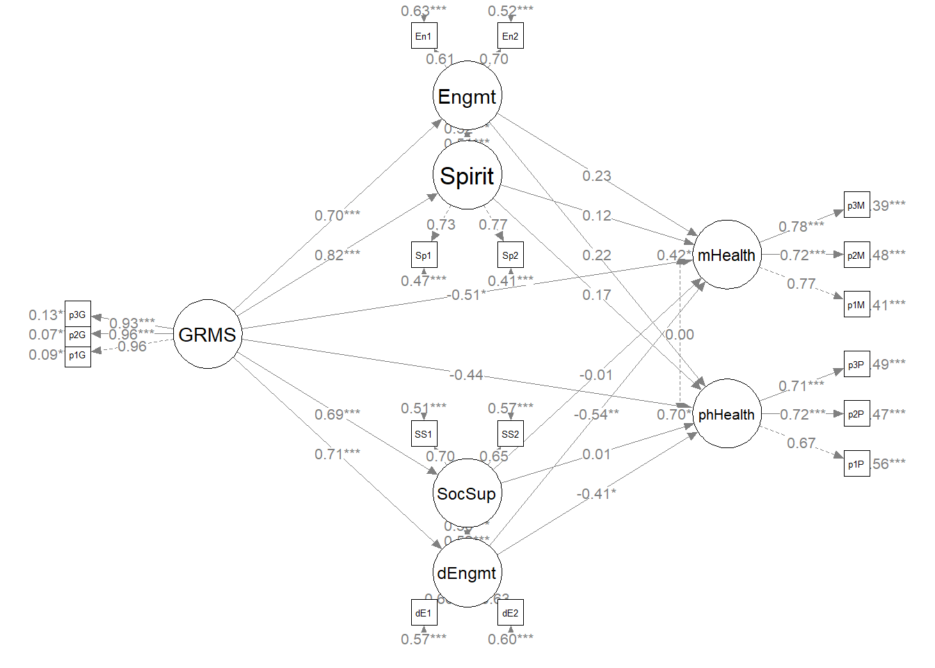
It can be useful to have a representation of the model without the results. This set of code produces those results. It does so by including only the name of the fitted object into the semPlot::semPaths function. Then it uses all the objects we just created as instructions for the figure’s appearance.
# Code to plot the theoretical model (in case you don't want to print
# the results on the graph):
plot1_theoretical <- semPlot::semPaths(struct_fit1, sizeMan = 3, node.width = 1,
    edge.label.cex = 0.75, style = "lisrel", mar = c(2, 2, 2, 2), structural = FALSE,
    curve = FALSE, intercepts = FALSE)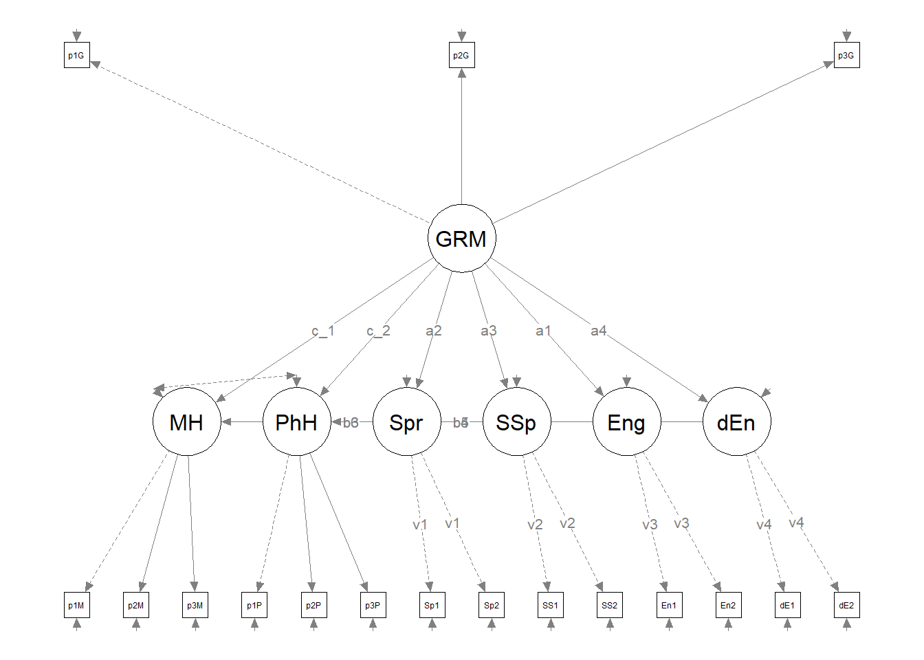
plot1_theoretical <- semptools::set_sem_layout(plot1_theoretical, indicator_order = m1_indicator_order,
    indicator_factor = m1_indicator_factor, factor_layout = m1_msmt, factor_point_to = m1_point_to,
    indicator_push = m1_indicator_push, indicator_spread = m1_indicator_spread)
plot(plot1_theoretical)
The statistical string for the global fit indices can be represented this way: \(\chi^2(109) = 120.324, p = 0.216, CFI = 0.994, RMSEA = 0.021, 90CI[0.000, 0.041], SRMR = 0.044\).
Tabling the regression weights will assist us in understanding the relations between the variables. To be consistent with my figure, in this table I have included the standardized results (i.e., \(\beta\)).
Table 2
| Model Coefficients Assessing the Effect of Gendered Racial Microaggressions on Mental and Physical Health through Coping Strategies |
|---|
| Predictor | \(B\) | \(SE_{B}\) | \(p\) | \(\beta\) | \(R^2\) |
|---|---|---|---|---|---|
| Engagement (M1) | .49 | ||||
| Gendered Racial Microaggressions (\(a_1\)) | 0.392 | 0.041 | < 0.001 | 0.701 | |
| Spirituality (M2) | .68 | ||||
| Gendered Racial Microaggressions (\(a_2\)) | 0.554 | 0.040 | < 0.001 | 0.824 | |
| Social Support (M3) | .48 | ||||
| Gendered Racial Microaggressions (\(a_3\)) | 0.406 | 0.042 | < 0.001 | 0.694 | |
| Disengagement (M4) | .50 | ||||
| Gendered Racial Microaggressions (\(a_4\)) | 0.386 | 0.041 | < 0.001 | 0.707 | |
| Mental Health (DV1) | .58 | ||||
| Engagement (\(b_1\)) | 0.355 | 0.223 | 0.111 | 0.229 | |
| Spirituality (\(b_1\)) | 0.155 | 0.219 | 0.481 | 0.120 | |
| Social Support (\(b_3\)) | -0.012 | 0.187 | 0.950 | -0.008 | |
| Disengagement (\(b_4\)) | -0.850 | 0.303 | 0.005 | -0.536 | |
| Gendered Racial Microaggressions (\(c'_1\)) | -0.445 | 0.205 | 0.029 | -0.514 | |
| Physical Health (DV2) | .30 | ||||
| Engagement (\(b_5\)) | 0.330 | 0.250 | 0.186 | 0.222 | |
| Spirituality (\(b_6\)) | 0.215 | 0.254 | 0.398 | 0.174 | |
| Social Support (\(b_7\)) | 0.016 | 0.215 | 0.939 | 0.012 | |
| Disengagement (\(b_8\)) | -0.624 | 0.295 | 0.034 | -0.409 | |
| Gendered Racial Microaggressions (\(c'_2\)) | -0.369 | 0.224 | 0.099 | -0.444 |
| Effects | \(B\) | \(SE_{B}\) | \(p\) | \(\beta\) | 95% CI |
|---|---|---|---|---|---|
| Indirect 3(\(a_1*b_1\)) | 0.139 | 0.089 | 0.118 | 0.161 | -0.035, 0.314 |
| Indirect 1(\(a_2*b_2\)) | 0.086 | 0.122 | 0.482 | 0.099 | -0.153, 0.325 |
| Indirect 2(\(a_3*b_3\)) | -0.005 | 0.076 | 0.950 | -0.005 | -0.154, 0.144 |
| Indirect 4(\(a_4*b_4\)) | -0.328 | 0.123 | 0.007 | -0.379 | -0.569, -0.088 |
| Direct 1 (\(c'_1\)) | -0.445 | 0.205 | 0.029 | -0.514 | -0.846, -0.045 |
| Total 1 (\(c_1\)) | -0.554 | 0.062 | < 0.001 | -0.639 | -0.675, -0.432 |
| Indirect 7(\(a_1*b_5\)) | 0.130 | 0.099 | 0.192 | 0.156 | -0.065, 0.324 |
| Indirect 5(\(a_2*b_6\)) | 0.119 | 0.141 | 0.400 | 0.143 | -0.158, 0.396 |
| Indirect 6(\(a_3*b_7\)) | 0.007 | 0.087 | 0.939 | 0.008 | -0.165, 0.178 |
| Indirect 8(\(a_4*b_8\)) | -0.241 | 0.117 | 0.039 | -0.289 | -0.470, -0.012 |
| Direct 2 (\(c'_2\)) | -0.369 | 0.224 | 0.099 | -0.444 | -0.808, 0.069 |
| Total 2 (\(c_2\)) | -0.394 | 0.083 | 0.000 | -0.445 | -0.556, -0.232 |
| Note. The significance of the indirect effects was calculated with bootstrapped, bias-corrected, confidence intervals (.95). |
As we can see, our model accounts for 48-68% of the variance in the mediators and 58% and 30% of the variance in the mental and physical health variables, respectively. Only one indirect effect, gendered racial microagressions to mental health, via disengagement coping. Inspection of the specific paths may provide some insight into this. Specifically, all of the a paths are statistically significant (i.e., gendered racial microaggressions predicting each of the four coping approaches) but only two of the b paths (i.e., disengagement coping to mental and physical health, respectively).
Here’s how I might write up this section of the analysis:
Our structural model was a parallel mediation, predicting mental and physical health directly from gendered racial microaggressions and indirectly through four coping strategies (i.e., spirituality, social support, engagement, disengagement). Results of the global fit indices suggested adequate fit \(\chi^2(109) = 120.324, p = 0.216, CFI = 0.994, RMSEA = 0.021, 90CI[0.000, 0.041], SRMR = 0.044\). As shown in Table 2 only two of the eight indirect effects was statistically significant. For both, disengagement coping mediated the effect of gendered racial microaggressions on mental health \((B = -0.328, p = 0.007)\) and physical health \((B = -0.241, p = 0.039)\). The model accunted for 48-68% of the variance in the mediators and 58% and 30% of the variance in mental and physical health, respectively.
With such strong overall fit, if I were the researcher, I would be inclined to stop here. Given that this is a lecture on model building and trimming, let’s proceed to see if respecification is indicated.
11.9 Model Building
Recall that in model building we start with a more parsimonious model and consider “adding paths.” This requires that our original model be overidentified with positive degrees of freedom. Earlier we determined that we had 8 degrees of freedom.
Modification indices are a tool that can help us determine where diretional paths or bidirectional covariances might improve model fit. A modification index is produced for each element of the model that is constrained to be zero (i.e., does not have a path or covariance). These modification indices are presented in the metric of the chi-square test and will tell us “by how much the chi-square value will decrease” if the two elements are freed to relate (i.e., by a path or covariance). In a one-degree chi-square test, statistically significant change occurs when the modification index is greater than 3.841. Thus, when researchers use the lavaan::modindices() function, they typically set a minimum value of 4.0 (rounding up from 3.841).
When inspecting the results, we will look for the parameters with the highest values (that are clearly above 4.0) that would be theoretically defensible. Be aware that this procedure may “suggest” many nonsensible relations.
##         lhs op     rhs     mi    epc sepc.lv sepc.all sepc.nox
## 125     PhH =~    p2MH 12.407  0.432   0.261    0.246    0.246
## 264    p2MH ~~   dEng2  8.859 -0.087  -0.087   -0.243   -0.243
## 362     SSp  ~     Spr  8.339  0.468   0.537    0.537    0.537
## 345     Spr ~~     SSp  8.339  0.036   0.422    0.422    0.422
## 357     Spr  ~     SSp  8.339  0.381   0.332    0.332    0.332
## 159     SSp =~ Spirit1  8.328  0.304   0.129    0.192    0.192
## 184    dEng =~    p2MH  7.683 -0.944  -0.374   -0.352   -0.352
## 303 Spirit1 ~~ Spirit2  7.539  2.239   2.239   11.841   11.841
## 325    Eng1 ~~    Eng2  7.538  0.635   0.635    2.853    2.853
## 372     PhH  ~      MH  7.538  0.453   0.471    0.471    0.471
## 330   dEng1 ~~   dEng2  7.538  0.140   0.140    0.639    0.639
## 32       MH ~~     PhH  7.538  0.074   0.363    0.363    0.363
## 371      MH  ~     PhH  7.538  0.292   0.280    0.280    0.280
## 133     PhH =~   dEng1  7.349  0.210   0.127    0.210    0.210
## 196  p1GRMS ~~  p3GRMS  7.107  0.022   0.022    0.384    0.384
## 245    p1MH ~~ Spirit1  6.205 -0.052  -0.052   -0.215   -0.215
## 119      MH =~   dEng1  6.170  0.186   0.117    0.194    0.194
## 241    p1MH ~~    p3MH  5.439  0.110   0.110    0.337    0.337
## 137     Spr =~  p3GRMS  5.237 -0.238  -0.116   -0.165   -0.165
## 185    dEng =~    p3MH  5.180  0.758   0.300    0.301    0.301
## 232  p3GRMS ~~ Spirit1  5.110 -0.022  -0.022   -0.188   -0.188
## 221  p2GRMS ~~   SocS2  5.098  0.022   0.022    0.213    0.213
## 351     Eng  ~     Spr  4.830  0.351   0.421    0.421    0.421
## 346     Spr ~~     Eng  4.830  0.027   0.334    0.334    0.334
## 356     Spr  ~     Eng  4.830  0.318   0.265    0.265    0.265
## 304 Spirit1 ~~   SocS1  4.473  0.036   0.036    0.183    0.183
## 16     dEng =~   dEng1  4.197 -0.290  -0.115   -0.191   -0.191
## 17     dEng =~   dEng2  4.197  0.290   0.115    0.183    0.183
Because we used the command, “sort=TRUE” the modification indices (in the “mi” column) are presented from highest to lowest. Having familiarity with lavaan syntax can be useful in deciphering what is being suggested.
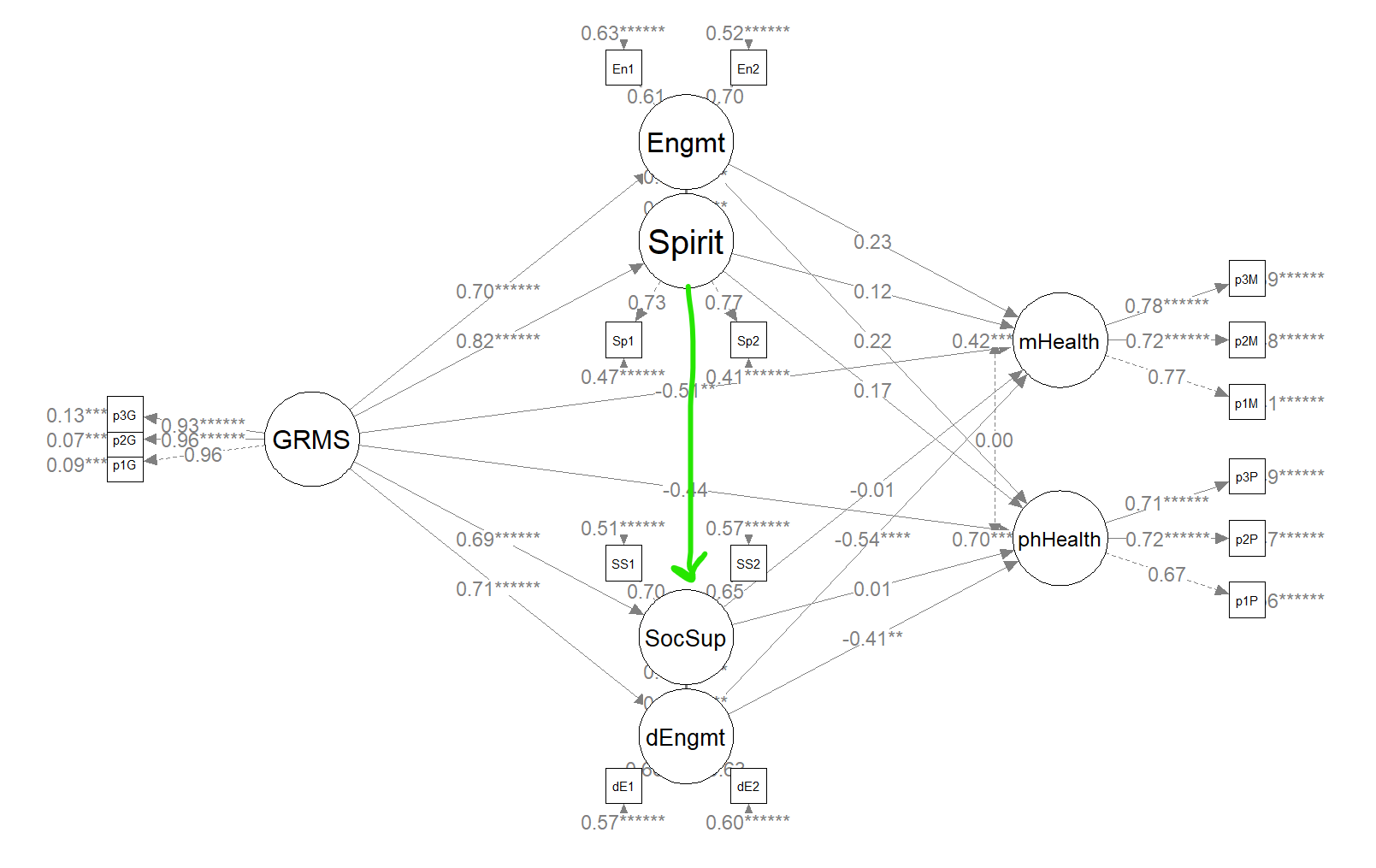
The first modification index (12.40) relates to the factor loadings in the measurement model. We know this because of the “=~” operator. It suggests that we free p2MH (the second parcel for mental health) to PhH (the physical health latent variable). I would consider this “nonsensible.” While this might improve model fit, this suggestion relates to our measurement model – and our measurement model had terrific fit with no need for further improvement.
The second modification index (8.859) is accompanied by the “~~” operator. This means it is suggesting that we free the second parcel for mental health to covary (correlate) with item 2 for disengagement coping. This is not a sensible suggestion. In fact the only sensible suggested covariation is to free the dependent variables (PhH and MH) to covary (correlate).
The single tilda (~) provides suggestions for regression paths. Note that the third and fifth recommendations are to either predict spiritual coping from social support coping or the vice versa. Further, the fourth recommendation is to allow those two variables to covary. Either of these three options would reduce our chi-square by 8.339. Keep in mind that the lavaan::modindices package will produce all possible combinations of ways to improve model fit, even if they are redundant.
I am intrigued by this suggested relation between spiritual coping and social support. If we added this path, we could test for the significance of an serially mediated effect from gendered racial microaggressions, to spiritual support, through social support, to mental and physical health, respectively.
struct_mod2 <- "
       ##measurement model
         GRMS =~ p1GRMS + p2GRMS + p3GRMS
         MH =~ p1MH + p2MH + p3MH
         PhH =~ p1PhH + p2PhH + p3PhH
         Spr =~ v1*Spirit1 + v1*Spirit2
         SSp =~ v2*SocS1 + v2*SocS2
         Eng =~ v3*Eng1 + v3*Eng2
         dEng =~ v4*dEng1 + v4*dEng2


        #structural model with labels for calculation of the indirect effect

         Eng ~ a1*GRMS
         Spr ~ a2*GRMS
         SSp ~ a3*GRMS
         dEng ~ a4*GRMS

         MH ~ c_p1*GRMS + b1*Eng + b2*Spr + b3*SSp + b4*dEng
         PhH ~ c_p2*GRMS  + b5*Eng + + b6*Spr + b7*SSp + b8*dEng

         SSp ~ d1*Spr

         #cov
         MH ~~ 0*PhH


        #calculations
         indirect.EngMH :=  a1*b1
         indirect.SprMH :=  a2*b2
         indirect.SSpMH :=  a3*b3
         indirect.dEngMH :=  a4*b4

         indirect.EngPhH :=  a1*b5
         indirect.SprPhH :=  a2*b6
         indirect.SSpPhH :=  a3*b7
         indirect.dEngPhH :=  a4*b8

         serial.MH := a2*d1*b3
         serial.PH := a2*d1*b7

         direct.MH  := c_p1
         direct.PhH  := c_p2
         total.MH  := c_p1 + (a1*b1) + (a2*b2) + (a3*b3) + (a4*b4) + (a2*d1*b3)
         total.PhH  := c_p2 + (a1*b5) + (a1*b6) + (a1*b7) + (a1*b8) + (a2*d1*b7)

          "
set.seed(230916)  #needed for reproducibility especially when specifying bootstrapped confidence intervals
struct_fit2 <- lavaan::sem(struct_mod2, data = dfLewis, missing = "fiml")
struct_summary2 <- lavaan::summary(struct_fit2, fit.measures = TRUE, standardized = TRUE,
    rsq = TRUE)
struct_pEsts2 <- lavaan::parameterEstimates(struct_fit2, boot.ci.type = "bca.simple",
    standardized = TRUE)
struct_summary2
## lavaan 0.6.17 ended normally after 121 iterations
##
## Estimator ML
## Optimization method NLMINB
## Number of model parameters 62
##
## Number of observations 231
## Number of missing patterns 1
##
## Model Test User Model:
##
## Test statistic 111.657
## Degrees of freedom 108
## P-value (Chi-square) 0.385
##
## Model Test Baseline Model:
##
## Test statistic 2104.157
## Degrees of freedom 136
## P-value 0.000
##
## User Model versus Baseline Model:
##
## Comparative Fit Index (CFI) 0.998
## Tucker-Lewis Index (TLI) 0.998
##
## Robust Comparative Fit Index (CFI) 0.998
## Robust Tucker-Lewis Index (TLI) 0.998
##
## Loglikelihood and Information Criteria:
##
## Loglikelihood user model (H0) -3385.514
## Loglikelihood unrestricted model (H1) -3329.686
##
## Akaike (AIC) 6895.029
## Bayesian (BIC) 7108.458
## Sample-size adjusted Bayesian (SABIC) 6911.954
##
## Root Mean Square Error of Approximation:
##
## RMSEA 0.012
## 90 Percent confidence interval - lower 0.000
## 90 Percent confidence interval - upper 0.036
## P-value H_0: RMSEA <= 0.050 0.999
## P-value H_0: RMSEA >= 0.080 0.000
##
## Robust RMSEA 0.012
## 90 Percent confidence interval - lower 0.000
## 90 Percent confidence interval - upper 0.036
## P-value H_0: Robust RMSEA <= 0.050 0.999
## P-value H_0: Robust RMSEA >= 0.080 0.000
##
## Standardized Root Mean Square Residual:
##
## SRMR 0.042
##
## Parameter Estimates:
##
## Standard errors Standard
## Information Observed
## Observed information based on Hessian
##
## Latent Variables:
## Estimate Std.Err z-value P(>|z|) Std.lv Std.all
## GRMS =~
## p1GRMS 1.000 0.725 0.955
## p2GRMS 1.014 0.030 34.076 0.000 0.736 0.962
## p3GRMS 0.903 0.030 29.918 0.000 0.655 0.933
## MH =~
## p1MH 1.000 0.628 0.769
## p2MH 1.217 0.126 9.664 0.000 0.765 0.721
## p3MH 1.245 0.113 11.045 0.000 0.783 0.783
## PhH =~
## p1PhH 1.000 0.604 0.666
## p2PhH 1.006 0.128 7.878 0.000 0.608 0.725
## p3PhH 1.036 0.135 7.662 0.000 0.626 0.715
## Spr =~
## Spirit1 (v1) 1.000 0.487 0.731
## Spirit2 (v1) 1.000 0.487 0.759
## SSp =~
## SocS1 (v2) 1.000 0.425 0.704
## SocS2 (v2) 1.000 0.425 0.654
## Eng =~
## Eng1 (v3) 1.000 0.406 0.607
## Eng2 (v3) 1.000 0.406 0.696
## dEng =~
## dEng1 (v4) 1.000 0.396 0.658
## dEng2 (v4) 1.000 0.396 0.633
##
## Regressions:
## Estimate Std.Err z-value P(>|z|) Std.lv Std.all
## Eng ~
## GRMS (a1) 0.392 0.041 9.498 0.000 0.700 0.700
## Spr ~
## GRMS (a2) 0.552 0.040 13.784 0.000 0.822 0.822
## SSp ~
## GRMS (a3) 0.138 0.109 1.266 0.205 0.236 0.236
## dEng ~
## GRMS (a4) 0.386 0.041 9.400 0.000 0.707 0.707
## MH ~
## GRMS (c_p1) -0.431 0.193 -2.236 0.025 -0.498 -0.498
## Eng (b1) 0.351 0.222 1.579 0.114 0.227 0.227
## Spr (b2) 0.185 0.277 0.668 0.504 0.144 0.144
## SSp (b3) -0.082 0.237 -0.347 0.729 -0.055 -0.055
## dEng (b4) -0.852 0.303 -2.815 0.005 -0.537 -0.537
## PhH ~
## GRMS (c_p2) -0.354 0.210 -1.690 0.091 -0.425 -0.425
## Eng (b5) 0.325 0.249 1.303 0.192 0.219 0.219
## Spr (b6) 0.257 0.322 0.797 0.425 0.207 0.207
## SSp (b7) -0.071 0.273 -0.259 0.795 -0.050 -0.050
## dEng (b8) -0.626 0.294 -2.129 0.033 -0.411 -0.411
## SSp ~
## Spr (d1) 0.477 0.180 2.646 0.008 0.548 0.548
##
## Covariances:
## Estimate Std.Err z-value P(>|z|) Std.lv Std.all
## .MH ~~
## .PhH 0.000 0.000 0.000
##
## Intercepts:
## Estimate Std.Err z-value P(>|z|) Std.lv Std.all
## .p1GRMS 2.592 0.050 51.897 0.000 2.592 3.415
## .p2GRMS 2.545 0.050 50.567 0.000 2.545 3.327
## .p3GRMS 2.579 0.046 55.829 0.000 2.579 3.673
## .p1MH 3.582 0.054 66.611 0.000 3.582 4.383
## .p2MH 2.866 0.070 41.023 0.000 2.866 2.699
## .p3MH 3.035 0.066 46.140 0.000 3.035 3.036
## .p1PhH 3.128 0.060 52.384 0.000 3.128 3.447
## .p2PhH 2.652 0.055 48.056 0.000 2.652 3.162
## .p3PhH 3.067 0.058 53.258 0.000 3.067 3.504
## .Spirit1 2.511 0.044 57.292 0.000 2.511 3.770
## .Spirit2 2.437 0.042 57.677 0.000 2.437 3.795
## .SocS1 2.550 0.040 64.289 0.000 2.550 4.230
## .SocS2 2.758 0.043 64.537 0.000 2.758 4.246
## .Eng1 2.437 0.044 55.375 0.000 2.437 3.643
## .Eng2 2.515 0.038 65.530 0.000 2.515 4.312
## .dEng1 2.502 0.040 63.177 0.000 2.502 4.157
## .dEng2 2.455 0.041 59.612 0.000 2.455 3.922
##
## Variances:
## Estimate Std.Err z-value P(>|z|) Std.lv Std.all
## .p1GRMS 0.050 0.007 6.695 0.000 0.050 0.087
## .p2GRMS 0.044 0.007 6.058 0.000 0.044 0.075
## .p3GRMS 0.064 0.008 8.355 0.000 0.064 0.129
## .p1MH 0.273 0.037 7.377 0.000 0.273 0.409
## .p2MH 0.542 0.067 8.062 0.000 0.542 0.481
## .p3MH 0.387 0.055 7.083 0.000 0.387 0.387
## .p1PhH 0.459 0.058 7.914 0.000 0.459 0.557
## .p2PhH 0.334 0.049 6.824 0.000 0.334 0.475
## .p3PhH 0.375 0.054 6.984 0.000 0.375 0.489
## .Spirit1 0.206 0.026 8.020 0.000 0.206 0.465
## .Spirit2 0.175 0.024 7.399 0.000 0.175 0.424
## .SocS1 0.183 0.025 7.198 0.000 0.183 0.504
## .SocS2 0.241 0.029 8.222 0.000 0.241 0.573
## .Eng1 0.282 0.033 8.560 0.000 0.282 0.631
## .Eng2 0.175 0.026 6.694 0.000 0.175 0.515
## .dEng1 0.205 0.029 7.123 0.000 0.205 0.567
## .dEng2 0.235 0.030 7.705 0.000 0.235 0.599
## GRMS 0.526 0.054 9.790 0.000 1.000 1.000
## .MH 0.164 0.042 3.926 0.000 0.416 0.416
## .PhH 0.255 0.058 4.392 0.000 0.698 0.698
## .Spr 0.077 0.019 4.044 0.000 0.324 0.324
## .SSp 0.078 0.022 3.576 0.000 0.431 0.431
## .Eng 0.084 0.022 3.819 0.000 0.510 0.510
## .dEng 0.078 0.024 3.333 0.001 0.500 0.500
##
## R-Square:
## Estimate
## p1GRMS 0.913
## p2GRMS 0.925
## p3GRMS 0.871
## p1MH 0.591
## p2MH 0.519
## p3MH 0.613
## p1PhH 0.443
## p2PhH 0.525
## p3PhH 0.511
## Spirit1 0.535
## Spirit2 0.576
## SocS1 0.496
## SocS2 0.427
## Eng1 0.369
## Eng2 0.485
## dEng1 0.433
## dEng2 0.401
## MH 0.584
## PhH 0.302
## Spr 0.676
## SSp 0.569
## Eng 0.490
## dEng 0.500
##
## Defined Parameters:
## Estimate Std.Err z-value P(>|z|) Std.lv Std.all
## indirect.EngMH 0.138 0.089 1.549 0.121 0.159 0.159
## indirect.SprMH 0.102 0.154 0.667 0.505 0.118 0.118
## indirect.SSpMH -0.011 0.032 -0.350 0.726 -0.013 -0.013
## indirct.dEngMH -0.329 0.122 -2.691 0.007 -0.380 -0.380
## indirct.EngPhH 0.127 0.099 1.287 0.198 0.153 0.153
## indirct.SprPhH 0.142 0.178 0.794 0.427 0.170 0.170
## indirct.SSpPhH -0.010 0.037 -0.264 0.792 -0.012 -0.012
## indrct.dEngPhH -0.242 0.117 -2.072 0.038 -0.290 -0.290
## serial.MH -0.022 0.064 -0.336 0.737 -0.025 -0.025
## serial.PH -0.019 0.074 -0.253 0.800 -0.022 -0.022
## direct.MH -0.431 0.193 -2.236 0.025 -0.498 -0.498
## direct.PhH -0.354 0.210 -1.690 0.091 -0.425 -0.425
## total.MH -0.554 0.062 -8.934 0.000 -0.639 -0.639
## total.PhH -0.418 0.134 -3.120 0.002 -0.472 -0.472# struct_pEsts2 #although creating the object is useful to export as
# a .csv I didn't ask it to print into the bookCreating a figure will help us with the conceptual understanding of what we’ve just done (and will also help us check our work).
Let’s first create a fresh plot from se
plot_struct2 <- semPlot::semPaths(struct_fit2, what = "col", whatLabels = "stand",
    sizeMan = 3, node.width = 1, edge.label.cex = 0.75, style = "lisrel",
    mar = c(2, 2, 2, 2), structural = FALSE, curve = FALSE, intercepts = FALSE)
Because we haven’t added or deleted variables (only 1 path) and we want them to stay in the same location with the same orientation of paths and covariances, we should be able to recycle some of the diagram code we created earlier
plot2 <- semptools::set_sem_layout(plot_struct2, indicator_order = m1_indicator_order,
    indicator_factor = m1_indicator_factor, factor_layout = m1_msmt, factor_point_to = m1_point_to,
    indicator_push = m1_indicator_push, indicator_spread = m1_indicator_spread)

# changing node labels
plot2 <- semptools::change_node_label(plot2, c(GRM = "GRMS", MH = "mHealth",
    PhH = "phHealth", Eng = "Engmt", dEn = "dEngmt", Spr = "Spirit", SSp = "SocSup"),
    label.cex = 1.1)

# adding stars to indicate significant paths
plot2 <- semptools::mark_sig(plot2, struct_fit2)

plot(plot2)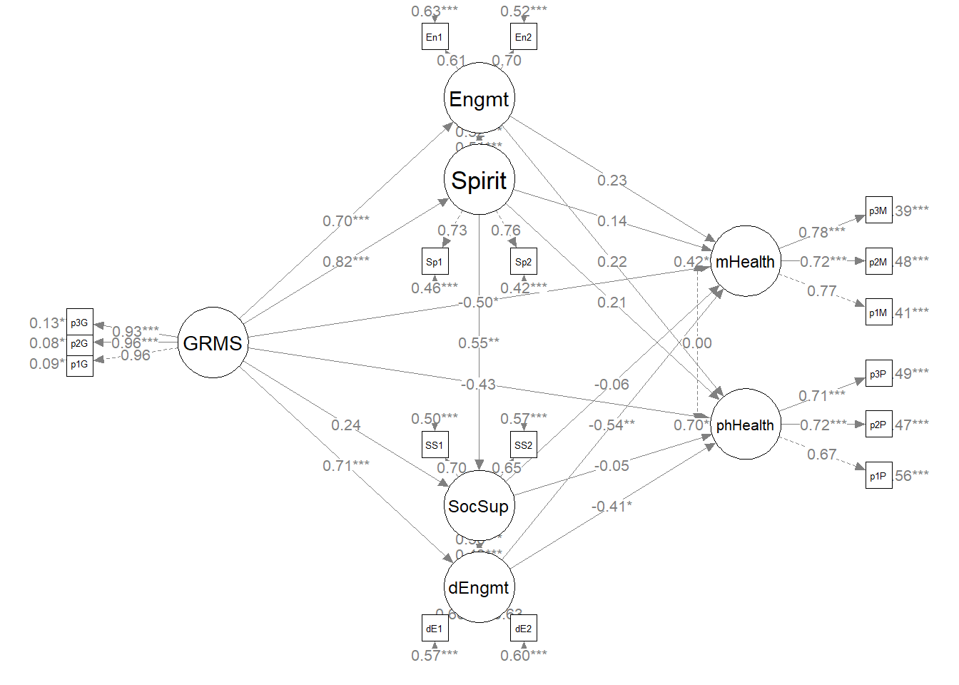
As predicted by the modification indices (and our knowledge that a model with fewer degrees of freedom will generally have improved fit), the global fit indices have improved: \(\chi^2(108) = 111.657, p = 0.385, CFI = 0.998, RMSEA = 0.012, 90CI[0.000, 0.036], SRMR = 0.042\)
We can formally compare these with the lavaan::lavTestLRT() function.
##
## Chi-Squared Difference Test
##
##              Df    AIC    BIC  Chisq Chisq diff   RMSEA Df diff Pr(>Chisq)
## struct_fit2 108 6895.0 7108.5 111.66
## struct_fit1 109 6901.7 7111.7 120.32      8.667 0.18218       1    0.00324 **
## ---
## Signif. codes:  0 '***' 0.001 '**' 0.01 '*' 0.05 '.' 0.1 ' ' 1
The chi-square difference test can be used to compare nested models. Models are nested when there is only the addition/deletion of paths or covariances. If the sample or variables change, they cannot be used. Our chi-square difference test was, \(\Delta\chi^2(1) = 8.667, p = 0.032\). This suggests that there were statistically significant difference in our nested models, favoring the newer model.
Something about this should look suspiciously familiar. Do you notice the chi-square value itself? Earlier our modification indices told us that if we freed Spr and SSp to relate, the chi-square value would drop by 8.339. While not exact, the prediction was fairly spot on!
Additionally, the AIC and BIC can be used to compare non-nested models. Preferred models have lower values. In our case, the newer model appears to be preferred.
Is freeing this parameter an appropriate addition to our model, or is it overparameterization. We should also inspect the \(d_1\) path and the serially mediated indirect effects. It does appear that regression weight from spirituality to social support (i.e., \(d_1\)) was statistically significant \((B = 0.477, p = 0.008)\) but the serially mediated indirect effects was not. Specifically, when mental health was the outcome, \(B = 0.022, p = 0.737\); when physical health was the outcome, \(B = -0.019, p = 0.800\).
Adding this path feels, to me, like overparameterization. In the case of model building, I will stick with the originally hypothesized model.
11.10 Model Trimming
In model trimming, the researcher starts with a more general model or saturated (i.e., zero degrees of freedom in the structural model) and, on the basis of statistical criteria, trims non-significant (i.e., and low regression weight) paths from the model. Chou and Bentler (2002) termed this backward searching. We have a number of non-significant paths. Should we delete them? And if so, how many of them?
The inclusion of indirect effects in our model makes it a little tricky to know how and where we might delete paths. As we look at the regression weights of our original model, I note that
- all b paths (except those involving disengagement coping) are non-significant,
- all indirect effects (except those involving disengagement coping) are non-significant,
- the b paths involving engagement coping are closest to being statistically significant.
It is a best practice to trim paths one at a time and then re-check the results. Why? Because the constraint may free up a little power and statistical significance for a regression path may turn on elsewhere. Because this is a book chapter and constraining each non-significant effect one-at-a-time would (a) take forever and (b) make this chapter absolutely unwieldy, I will first delete the b paths associated with social support at the same time. So that I can keep track of what I’m doing in my code, I will hashtag them out. The elimination of these will also result in the elimination of the associated indirect effect; I will hashtag those out, also.
struct_mod3 <- "
 ##measurement model
         GRMS =~ p1GRMS + p2GRMS + p3GRMS
         MH =~ p1MH + p2MH + p3MH
         PhH =~ p1PhH + p2PhH + p3PhH
         Spr =~ v1*Spirit1 + v1*Spirit2
         SSp =~ v2*SocS1 + v2*SocS2
         Eng =~ v3*Eng1 + v3*Eng2
         dEng =~ v4*dEng1 + v4*dEng2

         #structural model with labels for calculation of the indirect effect

         Eng ~ a1*GRMS
         Spr ~ a2*GRMS
         SSp ~ a3*GRMS
         dEng ~ a4*GRMS

         MH ~ c_p1*GRMS + b1*Eng + b2*Spr + b4*dEng #trimming + b3*SSp
         PhH ~ c_p2*GRMS  + b5*Eng + + b6*Spr + b8*dEng #trimming + b7*SSp

         #cov
         MH ~~ 0*PhH #prevents MH and PhD from correlating

        #calculations
         indirect.EngMH :=  a1*b1
         indirect.SprMH :=  a2*b2
         #indirect.SSpMH :=  a3*b3 #trimmed after deleting b3, above
         indirect.dEngMH :=  a4*b4

         indirect.EngPhH :=  a1*b5
         indirect.SprPhH :=  a2*b6
         #indirect.SSpPhH :=  a3*b7 #trimmed after deleting b7, above
         indirect.dEngPhH :=  a4*b8
         direct.MH  := c_p1
         direct.PhH  := c_p2
         total.MH  := c_p1 + (a1*b1) + (a2*b2)  + (a4*b4) #trimmed + (a3*b3)
         total.PhH  := c_p2 + (a1*b5) + (a1*b6) + (a1*b8) #trimmed + (a1*b7)

          "
set.seed(230916)  #needed for reproducibility especially when specifying bootstrapped confidence intervals
struct_fit3 <- lavaan::sem(struct_mod3, data = dfLewis, missing = "fiml")
struct_summary3 <- lavaan::summary(struct_fit3, fit.measures = TRUE, standardized = TRUE,
    rsq = TRUE)
struct_pEsts3 <- lavaan::parameterEstimates(struct_fit3, boot.ci.type = "bca.simple",
    standardized = TRUE)
struct_summary3
## lavaan 0.6.17 ended normally after 113 iterations
##
## Estimator ML
## Optimization method NLMINB
## Number of model parameters 61
##
## Number of observations 231
## Number of missing patterns 1
##
## Model Test User Model:
##
## Test statistic 120.319
## Degrees of freedom 109
## P-value (Chi-square) 0.216
##
## Model Test Baseline Model:
##
## Test statistic 2104.157
## Degrees of freedom 136
## P-value 0.000
##
## User Model versus Baseline Model:
##
## Comparative Fit Index (CFI) 0.994
## Tucker-Lewis Index (TLI) 0.993
##
## Robust Comparative Fit Index (CFI) 0.994
## Robust Tucker-Lewis Index (TLI) 0.993
##
## Loglikelihood and Information Criteria:
##
## Loglikelihood user model (H0) -3389.845
## Loglikelihood unrestricted model (H1) -3329.686
##
## Akaike (AIC) 6901.691
## Bayesian (BIC) 7111.678
## Sample-size adjusted Bayesian (SABIC) 6918.343
##
## Root Mean Square Error of Approximation:
##
## RMSEA 0.021
## 90 Percent confidence interval - lower 0.000
## 90 Percent confidence interval - upper 0.041
## P-value H_0: RMSEA <= 0.050 0.995
## P-value H_0: RMSEA >= 0.080 0.000
##
## Robust RMSEA 0.021
## 90 Percent confidence interval - lower 0.000
## 90 Percent confidence interval - upper 0.041
## P-value H_0: Robust RMSEA <= 0.050 0.995
## P-value H_0: Robust RMSEA >= 0.080 0.000
##
## Standardized Root Mean Square Residual:
##
## SRMR 0.044
##
## Parameter Estimates:
##
## Standard errors Standard
## Information Observed
## Observed information based on Hessian
##
## Latent Variables:
## Estimate Std.Err z-value P(>|z|) Std.lv Std.all
## GRMS =~
## p1GRMS 1.000 0.725 0.955
## p2GRMS 1.015 0.030 34.097 0.000 0.736 0.962
## p3GRMS 0.903 0.030 29.818 0.000 0.655 0.932
## MH =~
## p1MH 1.000 0.628 0.769
## p2MH 1.218 0.126 9.662 0.000 0.765 0.721
## p3MH 1.245 0.113 11.045 0.000 0.783 0.783
## PhH =~
## p1PhH 1.000 0.604 0.666
## p2PhH 1.007 0.128 7.878 0.000 0.608 0.725
## p3PhH 1.035 0.135 7.664 0.000 0.625 0.714
## Spr =~
## Spirit1 (v1) 1.000 0.488 0.726
## Spirit2 (v1) 1.000 0.488 0.766
## SSp =~
## SocS1 (v2) 1.000 0.425 0.703
## SocS2 (v2) 1.000 0.425 0.655
## Eng =~
## Eng1 (v3) 1.000 0.406 0.607
## Eng2 (v3) 1.000 0.406 0.696
## dEng =~
## dEng1 (v4) 1.000 0.396 0.658
## dEng2 (v4) 1.000 0.396 0.633
##
## Regressions:
## Estimate Std.Err z-value P(>|z|) Std.lv Std.all
## Eng ~
## GRMS (a1) 0.392 0.041 9.506 0.000 0.701 0.701
## Spr ~
## GRMS (a2) 0.554 0.040 13.869 0.000 0.824 0.824
## SSp ~
## GRMS (a3) 0.406 0.042 9.685 0.000 0.694 0.694
## dEng ~
## GRMS (a4) 0.386 0.041 9.400 0.000 0.707 0.707
## MH ~
## GRMS (c_p1) -0.450 0.193 -2.336 0.019 -0.520 -0.520
## Eng (b1) 0.355 0.222 1.594 0.111 0.229 0.229
## Spr (b2) 0.156 0.218 0.712 0.476 0.121 0.121
## dEng (b4) -0.850 0.303 -2.807 0.005 -0.536 -0.536
## PhH ~
## GRMS (c_p2) -0.363 0.209 -1.735 0.083 -0.435 -0.435
## Eng (b5) 0.330 0.249 1.325 0.185 0.222 0.222
## Spr (b6) 0.214 0.253 0.845 0.398 0.173 0.173
## dEng (b8) -0.623 0.295 -2.115 0.034 -0.409 -0.409
##
## Covariances:
## Estimate Std.Err z-value P(>|z|) Std.lv Std.all
## .MH ~~
## .PhH 0.000 0.000 0.000
## .SSp -0.002 0.017 -0.094 0.925 -0.013 -0.013
## .PhH ~~
## .SSp 0.002 0.019 0.104 0.917 0.013 0.013
##
## Intercepts:
## Estimate Std.Err z-value P(>|z|) Std.lv Std.all
## .p1GRMS 2.592 0.050 51.897 0.000 2.592 3.415
## .p2GRMS 2.545 0.050 50.567 0.000 2.545 3.327
## .p3GRMS 2.579 0.046 55.829 0.000 2.579 3.673
## .p1MH 3.582 0.054 66.613 0.000 3.582 4.383
## .p2MH 2.866 0.070 41.024 0.000 2.866 2.699
## .p3MH 3.035 0.066 46.141 0.000 3.035 3.036
## .p1PhH 3.128 0.060 52.389 0.000 3.128 3.447
## .p2PhH 2.652 0.055 48.062 0.000 2.652 3.162
## .p3PhH 3.067 0.058 53.264 0.000 3.067 3.504
## .Spirit1 2.511 0.044 56.810 0.000 2.511 3.738
## .Spirit2 2.437 0.042 58.201 0.000 2.437 3.829
## .SocS1 2.550 0.040 64.171 0.000 2.550 4.222
## .SocS2 2.758 0.043 64.666 0.000 2.758 4.255
## .Eng1 2.437 0.044 55.380 0.000 2.437 3.644
## .Eng2 2.515 0.038 65.524 0.000 2.515 4.311
## .dEng1 2.502 0.040 63.179 0.000 2.502 4.157
## .dEng2 2.455 0.041 59.610 0.000 2.455 3.922
##
## Variances:
## Estimate Std.Err z-value P(>|z|) Std.lv Std.all
## .p1GRMS 0.050 0.007 6.754 0.000 0.050 0.087
## .p2GRMS 0.044 0.007 6.098 0.000 0.044 0.075
## .p3GRMS 0.064 0.008 8.400 0.000 0.064 0.131
## .p1MH 0.273 0.037 7.378 0.000 0.273 0.409
## .p2MH 0.542 0.067 8.059 0.000 0.542 0.481
## .p3MH 0.387 0.055 7.083 0.000 0.387 0.387
## .p1PhH 0.459 0.058 7.915 0.000 0.459 0.557
## .p2PhH 0.333 0.049 6.816 0.000 0.333 0.474
## .p3PhH 0.375 0.054 6.997 0.000 0.375 0.490
## .Spirit1 0.214 0.026 8.135 0.000 0.214 0.473
## .Spirit2 0.167 0.023 7.223 0.000 0.167 0.413
## .SocS1 0.184 0.026 7.154 0.000 0.184 0.506
## .SocS2 0.240 0.029 8.139 0.000 0.240 0.571
## .Eng1 0.282 0.033 8.558 0.000 0.282 0.631
## .Eng2 0.175 0.026 6.695 0.000 0.175 0.515
## .dEng1 0.205 0.029 7.116 0.000 0.205 0.567
## .dEng2 0.235 0.030 7.702 0.000 0.235 0.599
## GRMS 0.526 0.054 9.787 0.000 1.000 1.000
## .MH 0.164 0.042 3.929 0.000 0.416 0.416
## .PhH 0.255 0.058 4.403 0.000 0.700 0.700
## .Spr 0.076 0.019 4.051 0.000 0.321 0.321
## .SSp 0.094 0.021 4.414 0.000 0.519 0.519
## .Eng 0.084 0.022 3.809 0.000 0.509 0.509
## .dEng 0.078 0.024 3.332 0.001 0.500 0.500
##
## R-Square:
## Estimate
## p1GRMS 0.913
## p2GRMS 0.925
## p3GRMS 0.869
## p1MH 0.591
## p2MH 0.519
## p3MH 0.613
## p1PhH 0.443
## p2PhH 0.526
## p3PhH 0.510
## Spirit1 0.527
## Spirit2 0.587
## SocS1 0.494
## SocS2 0.429
## Eng1 0.369
## Eng2 0.485
## dEng1 0.433
## dEng2 0.401
## MH 0.584
## PhH 0.300
## Spr 0.679
## SSp 0.481
## Eng 0.491
## dEng 0.500
##
## Defined Parameters:
## Estimate Std.Err z-value P(>|z|) Std.lv Std.all
## indirect.EngMH 0.139 0.089 1.564 0.118 0.161 0.161
## indirect.SprMH 0.086 0.121 0.710 0.478 0.099 0.099
## indirct.dEngMH -0.329 0.122 -2.685 0.007 -0.379 -0.379
## indirct.EngPhH 0.130 0.099 1.307 0.191 0.156 0.156
## indirct.SprPhH 0.119 0.141 0.842 0.400 0.142 0.142
## indrct.dEngPhH -0.241 0.117 -2.060 0.039 -0.289 -0.289
## direct.MH -0.450 0.193 -2.336 0.019 -0.520 -0.520
## direct.PhH -0.363 0.209 -1.735 0.083 -0.435 -0.435
## total.MH -0.554 0.062 -8.932 0.000 -0.639 -0.639
## total.PhH -0.394 0.083 -4.752 0.000 -0.445 -0.445# struct_pEsts3 #although creating the object is useful to export as
# a .csv I didn't ask it to print into the bookCreating a figure will help us with the conceptual understanding of what we’ve just done (and will also help us check our work).
Let’s first create a fresh plot from se
plot_struct3 <- semPlot::semPaths(struct_fit3, what = "col", whatLabels = "stand",
    sizeMan = 3, node.width = 1, edge.label.cex = 0.75, style = "lisrel",
    mar = c(2, 2, 2, 2), structural = FALSE, curve = FALSE, intercepts = FALSE)
Because we haven’t added or deleted variables (only 1 path) and we want them to stay in the same location with the same orientation of paths and covariances, we should be able to recycle some of the diagram code we created earlier
plot3 <- semptools::set_sem_layout(plot_struct3, indicator_order = m1_indicator_order,
    indicator_factor = m1_indicator_factor, factor_layout = m1_msmt, factor_point_to = m1_point_to,
    indicator_push = m1_indicator_push, indicator_spread = m1_indicator_spread)

# changing node labels
plot3 <- semptools::change_node_label(plot3, c(GRM = "GRMS", MH = "mHealth",
    PhH = "phHealth", Eng = "Engmt", dEn = "dEngmt", Spr = "Spirit", SSp = "SocSup"),
    label.cex = 1.1)

# adding stars to indicate significant paths
plot3 <- semptools::mark_sig(plot3, struct_fit3)

plot(plot3)
Close inspection shows that there are no longer b paths from social support to mental and physical health.
Curiously, even though we deleted two paths, our degrees of freedom was the same as the original model. This means that our fit indices will be identical: \(\chi^2(109) = 120.319, p = 0.216, CFI = 0.994, RMSEA = 0.021, 90CI[0.000, 0.041], SRMR = 0.044\).
We can formally test differences in the two models with the lavaan:lavTestLRT() function.
## Warning in lavaan::lavTestLRT(struct_fit1, struct_fit3): lavaan WARNING:
##     Some restricted models fit better than less restricted models;
##     either these models are not nested, or the less restricted model
##     failed to reach a global optimum. Smallest difference =
##     -0.00500996567915024
## Warning in lavaan::lavTestLRT(struct_fit1, struct_fit3): lavaan WARNING: some
## models have the same degrees of freedom##
## Chi-Squared Difference Test
##
## Df AIC BIC Chisq Chisq diff RMSEA Df diff Pr(>Chisq)
## struct_fit1 109 6901.7 7111.7 120.32
## struct_fit3 109 6901.7 7111.7 120.32 -0.00501 0 0As shown, this df = 0 test indicated that the models are not statistically significantly different form each other.
When researchers engage in model trimming, their (typical) hope is that the models are not statistically significantly different from each other. Why? This means that the more parsimonious model (i.e., the nested model, the one with fewer paths/covariances) fits similarly to the sample covariance matrix (i.e., where all variables freely covary).
11.10.0.1 Extreme Model Trimming
In the description of the Lewis et al. (2017), I noted that the researchers conducted eight simple mediations instead of two parallel mediations (for mental and physical health, respectively), or as we have done – a complex SEM modeling all four mediators with both dependent variables. Given the small regression weights and very non-significant p values for spirituality and social support, I’m curious what would happen if we respecified the model, retaining only disengagement and engagement variables. This level of respecification would render our model as non-nested so our comparison would be limited to the AIC/BIC (lower values indicate better fit) and the global fit indices, themselves (without formal comparison).
struct_mod4 <- "
        ##measurement model
         GRMS =~ p1GRMS + p2GRMS + p3GRMS
         MH =~ p1MH + p2MH + p3MH
         PhH =~ p1PhH + p2PhH + p3PhH
         #Spr =~ v1*Spirit1 + v1*Spirit2 #trimmed altogether
         #SSp =~ v2*SocS1 + v2*SocS2 #trimmed altogether
         Eng =~ v3*Eng1 + v3*Eng2
         dEng =~ v4*dEng1 + v4*dEng2

         #structural model with labels for calculation of the indirect effect

         Eng ~ a1*GRMS
         #Spr ~ a2*GRMS #trimmed altogether
         #SSp ~ a3*GRMS #trimmed altogether
         dEng ~ a4*GRMS

         MH ~ c_p1*GRMS + b1*Eng + b4*dEng #trimming + b2*Spr + b3*SSp
         PhH ~ c_p2*GRMS  + b5*Eng  + b8*dEng #trimming + b6*Spr + b7*SSp

         #cov
         MH ~~ 0*PhH #prevents MH and PhD from correlating

        #calculations
         indirect.EngMH :=  a1*b1
         #indirect.SprMH :=  a2*b2 #trimmed after deleting Spr
         #indirect.SSpMH :=  a3*b3 #trimmed after deleting SSp
         indirect.dEngMH :=  a4*b4

         indirect.EngPhH :=  a1*b5
         #indirect.SprPhH :=  a2*b6 #trimmed after deleting Spr
         #indirect.SSpPhH :=  a3*b7 #trimmed after deleting Ssp
         indirect.dEngPhH :=  a4*b8
         direct.MH  := c_p1
         direct.PhH  := c_p2
         total.MH  := c_p1 + (a1*b1) + (a4*b4) #trimmed  + (a2*b2)  + (a3*b3)
         total.PhH  := c_p2 + (a1*b5) + (a1*b8) #trimmed + (a1*b6) + (a1*b7)

          "
set.seed(230916)  #needed for reproducibility especially when specifying bootstrapped confidence intervals
struct_fit4 <- lavaan::sem(struct_mod4, data = dfLewis, missing = "fiml")
struct_summary4 <- lavaan::summary(struct_fit4, fit.measures = TRUE, standardized = TRUE,
    rsq = TRUE)
struct_pEsts4 <- lavaan::parameterEstimates(struct_fit4, boot.ci.type = "bca.simple",
    standardized = TRUE)
struct_summary4
## lavaan 0.6.17 ended normally after 64 iterations
##
## Estimator ML
## Optimization method NLMINB
## Number of model parameters 45
##
## Number of observations 231
## Number of missing patterns 1
##
## Model Test User Model:
##
## Test statistic 59.999
## Degrees of freedom 59
## P-value (Chi-square) 0.439
##
## Model Test Baseline Model:
##
## Test statistic 1675.582
## Degrees of freedom 78
## P-value 0.000
##
## User Model versus Baseline Model:
##
## Comparative Fit Index (CFI) 0.999
## Tucker-Lewis Index (TLI) 0.999
##
## Robust Comparative Fit Index (CFI) 0.999
## Robust Tucker-Lewis Index (TLI) 0.999
##
## Loglikelihood and Information Criteria:
##
## Loglikelihood user model (H0) -2675.295
## Loglikelihood unrestricted model (H1) -2645.296
##
## Akaike (AIC) 5440.591
## Bayesian (BIC) 5595.500
## Sample-size adjusted Bayesian (SABIC) 5452.875
##
## Root Mean Square Error of Approximation:
##
## RMSEA 0.009
## 90 Percent confidence interval - lower 0.000
## 90 Percent confidence interval - upper 0.042
## P-value H_0: RMSEA <= 0.050 0.989
## P-value H_0: RMSEA >= 0.080 0.000
##
## Robust RMSEA 0.009
## 90 Percent confidence interval - lower 0.000
## 90 Percent confidence interval - upper 0.042
## P-value H_0: Robust RMSEA <= 0.050 0.989
## P-value H_0: Robust RMSEA >= 0.080 0.000
##
## Standardized Root Mean Square Residual:
##
## SRMR 0.043
##
## Parameter Estimates:
##
## Standard errors Standard
## Information Observed
## Observed information based on Hessian
##
## Latent Variables:
## Estimate Std.Err z-value P(>|z|) Std.lv Std.all
## GRMS =~
## p1GRMS 1.000 0.726 0.956
## p2GRMS 1.011 0.030 33.674 0.000 0.734 0.959
## p3GRMS 0.906 0.030 30.368 0.000 0.658 0.936
## MH =~
## p1MH 1.000 0.628 0.768
## p2MH 1.219 0.126 9.704 0.000 0.766 0.721
## p3MH 1.245 0.112 11.078 0.000 0.782 0.782
## PhH =~
## p1PhH 1.000 0.603 0.665
## p2PhH 1.008 0.128 7.879 0.000 0.608 0.725
## p3PhH 1.037 0.135 7.663 0.000 0.626 0.715
## Eng =~
## Eng1 (v3) 1.000 0.406 0.606
## Eng2 (v3) 1.000 0.406 0.695
## dEng =~
## dEng1 (v4) 1.000 0.396 0.658
## dEng2 (v4) 1.000 0.396 0.633
##
## Regressions:
## Estimate Std.Err z-value P(>|z|) Std.lv Std.all
## Eng ~
## GRMS (a1) 0.389 0.041 9.419 0.000 0.697 0.697
## dEng ~
## GRMS (a4) 0.385 0.041 9.351 0.000 0.705 0.705
## MH ~
## GRMS (c_p1) -0.374 0.161 -2.319 0.020 -0.432 -0.432
## Eng (b1) 0.373 0.220 1.692 0.091 0.241 0.241
## dEng (b4) -0.841 0.302 -2.784 0.005 -0.531 -0.531
## PhH ~
## GRMS (c_p2) -0.259 0.168 -1.541 0.123 -0.312 -0.312
## Eng (b5) 0.360 0.247 1.456 0.146 0.242 0.242
## dEng (b8) -0.611 0.294 -2.083 0.037 -0.401 -0.401
##
## Covariances:
## Estimate Std.Err z-value P(>|z|) Std.lv Std.all
## .MH ~~
## .PhH 0.000 0.000 0.000
##
## Intercepts:
## Estimate Std.Err z-value P(>|z|) Std.lv Std.all
## .p1GRMS 2.592 0.050 51.897 0.000 2.592 3.415
## .p2GRMS 2.545 0.050 50.567 0.000 2.545 3.327
## .p3GRMS 2.579 0.046 55.829 0.000 2.579 3.673
## .p1MH 3.582 0.054 66.626 0.000 3.582 4.384
## .p2MH 2.866 0.070 41.030 0.000 2.866 2.700
## .p3MH 3.035 0.066 46.150 0.000 3.035 3.036
## .p1PhH 3.128 0.060 52.387 0.000 3.128 3.447
## .p2PhH 2.652 0.055 48.059 0.000 2.652 3.162
## .p3PhH 3.067 0.058 53.261 0.000 3.067 3.504
## .Eng1 2.437 0.044 55.381 0.000 2.437 3.644
## .Eng2 2.515 0.038 65.523 0.000 2.515 4.311
## .dEng1 2.502 0.040 63.148 0.000 2.502 4.155
## .dEng2 2.455 0.041 59.634 0.000 2.455 3.924
##
## Variances:
## Estimate Std.Err z-value P(>|z|) Std.lv Std.all
## .p1GRMS 0.049 0.008 6.508 0.000 0.049 0.085
## .p2GRMS 0.047 0.008 6.191 0.000 0.047 0.080
## .p3GRMS 0.061 0.008 8.075 0.000 0.061 0.123
## .p1MH 0.273 0.037 7.431 0.000 0.273 0.410
## .p2MH 0.541 0.067 8.067 0.000 0.541 0.480
## .p3MH 0.388 0.055 7.098 0.000 0.388 0.388
## .p1PhH 0.459 0.058 7.923 0.000 0.459 0.558
## .p2PhH 0.333 0.049 6.821 0.000 0.333 0.474
## .p3PhH 0.374 0.054 6.993 0.000 0.374 0.489
## .Eng1 0.283 0.033 8.541 0.000 0.283 0.632
## .Eng2 0.176 0.026 6.668 0.000 0.176 0.517
## .dEng1 0.206 0.029 7.085 0.000 0.206 0.567
## .dEng2 0.234 0.031 7.671 0.000 0.234 0.599
## GRMS 0.527 0.054 9.803 0.000 1.000 1.000
## .MH 0.166 0.042 3.957 0.000 0.421 0.421
## .PhH 0.257 0.058 4.414 0.000 0.707 0.707
## .Eng 0.085 0.022 3.798 0.000 0.515 0.515
## .dEng 0.079 0.024 3.326 0.001 0.503 0.503
##
## R-Square:
## Estimate
## p1GRMS 0.915
## p2GRMS 0.920
## p3GRMS 0.877
## p1MH 0.590
## p2MH 0.520
## p3MH 0.612
## p1PhH 0.442
## p2PhH 0.526
## p3PhH 0.511
## Eng1 0.368
## Eng2 0.483
## dEng1 0.433
## dEng2 0.401
## MH 0.579
## PhH 0.293
## Eng 0.485
## dEng 0.497
##
## Defined Parameters:
## Estimate Std.Err z-value P(>|z|) Std.lv Std.all
## indirect.EngMH 0.145 0.088 1.656 0.098 0.168 0.168
## indirct.dEngMH -0.324 0.122 -2.662 0.008 -0.374 -0.374
## indirct.EngPhH 0.140 0.098 1.433 0.152 0.169 0.169
## indrct.dEngPhH -0.235 0.116 -2.029 0.043 -0.283 -0.283
## direct.MH -0.374 0.161 -2.319 0.020 -0.432 -0.432
## direct.PhH -0.259 0.168 -1.541 0.123 -0.312 -0.312
## total.MH -0.552 0.062 -8.930 0.000 -0.638 -0.638
## total.PhH -0.357 0.071 -5.054 0.000 -0.423 -0.423# struct_pEsts4 #although creating the object is useful to export as
# a .csv I didn't ask it to print into the bookCreating a figure to represent our analysis will require us to tweak the full set of code.
plot_struct4 <- semPlot::semPaths(struct_fit4, what = "col", whatLabels = "stand",
sizeMan = 3, node.width = 1, edge.label.cex = 0.75, style = "lisrel",
mar = c(2, 2, 2, 2), structural = FALSE, curve = FALSE, intercepts = FALSE)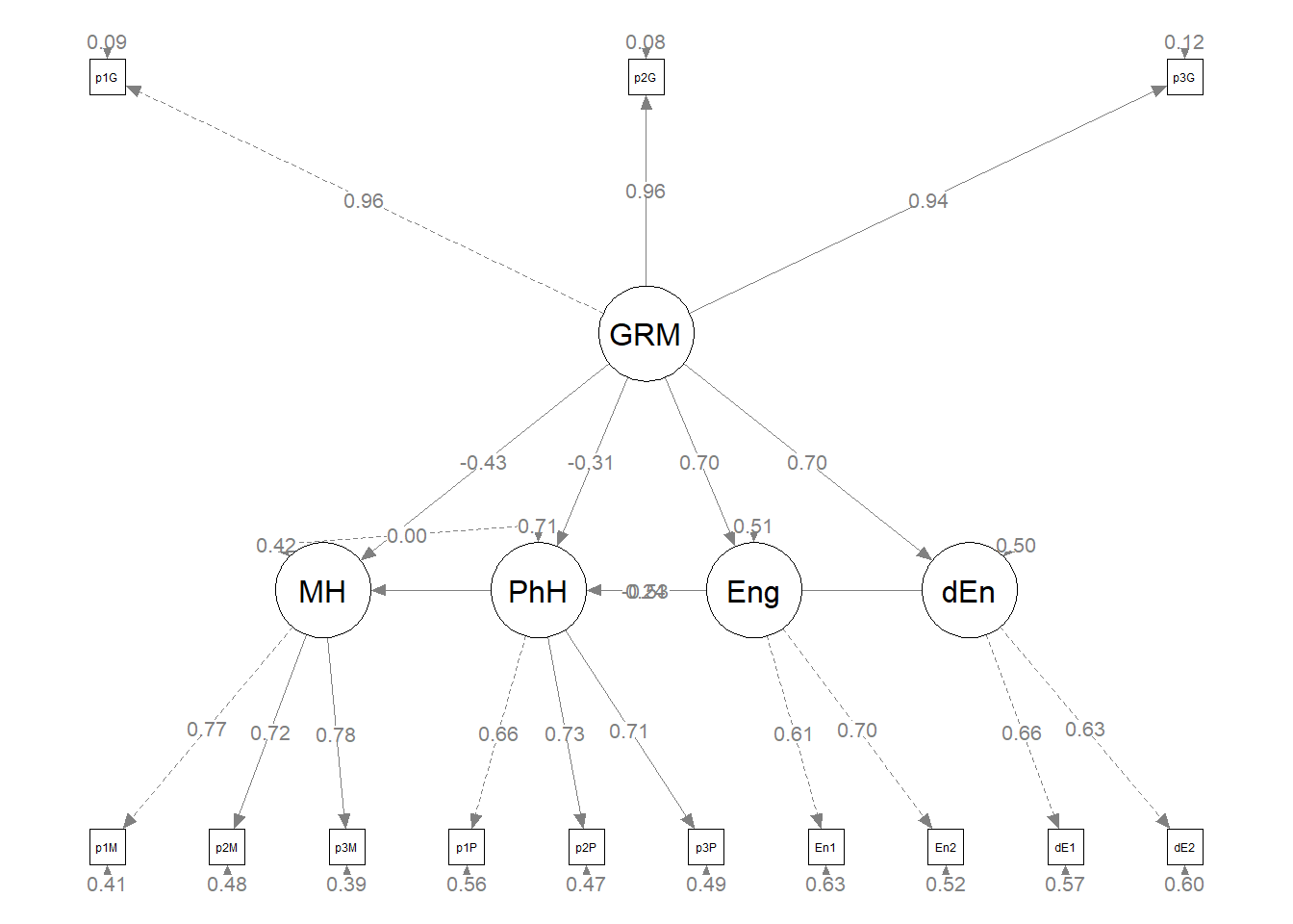 Although the code below may look daunting, I find it to be a fairly straightforward way to obtain figures that convey the model we are testing. We first start by identifying the desired location of our latent variables, using numbers to represent their position by “(column, row)”. In the table below, I have mapped my variables.
| Grid for Plotting semplot::sempath | ||
|---|---|---|
| (1,1) | (1,2) Eng | (1,3) |
| (2,1) | (2,2) | (2,3) MH |
| (3,1) GRM | (3,2) | (3,3) |
| (4,1) | (4,2) | (4,3) PhH |
| (5,1) | (5,2) dEn | (5,3) |
We place these values along with the names of our latent variables in to the semptools::layout_matrix function.
# IMPORTANT: Must use the node names (take directly from the SemPlot)
# assigned by SemPlot You can change them as the last thing
m4_msmt <- semptools::layout_matrix(GRM = c(3, 1), Eng = c(1, 2), dEn = c(5,
    2), MH = c(2, 3), PhH = c(4, 3))

# tell where you want the indicators to face
m4_point_to <- semptools::layout_matrix(left = c(3, 1), up = c(1, 2), down = c(5,
    2), right = c(2, 3), right = c(4, 3))

# the next two codes -- indicator_order and indicator_factor are
# paired together, they specify the order of observed variables for
# each factor
m4_indicator_order <- c("p1G", "p2G", "p3G", "p1M", "p2M", "p3M", "p1P",
    "p2P", "p3P", "En1", "En2", "dE1", "dE2")

m4_indicator_factor <- c("GRM", "GRM", "GRM", "MH", "MH", "MH", "PhH",
    "PhH", "PhH", "Eng", "Eng", "dEn", "dEn")

# next set of code pushes the indicator variables away from the
# factor
m4_indicator_push <- c(GRM = 0.5, MH = 1, PhH = 1, Eng = 1.5, dEn = 2)

# spreading the boxes away from each other
m4_indicator_spread <- c(GRM = 0.5, MH = 1, PhH = 1, Eng = 1, dEn = 1)

plot4 <- semptools::set_sem_layout(plot_struct4, indicator_order = m4_indicator_order,
    indicator_factor = m4_indicator_factor, factor_layout = m4_msmt, factor_point_to = m4_point_to,
    indicator_push = m4_indicator_push, indicator_spread = m4_indicator_spread)

# changing node labels -- throwing an error and I'm not sure why, it
# worked above plot4 <- semptools::change_node_label(plot4, c(GRM =
# 'GRMS', MH = 'mHealth', PhH = 'phHealth', Eng = 'Engmt', dEn =
# 'dEngmt', label.cex = 1.1))

# adding stars to indicate significant paths
plot4 <- semptools::mark_sig(plot4, struct_fit4)

plot(plot4)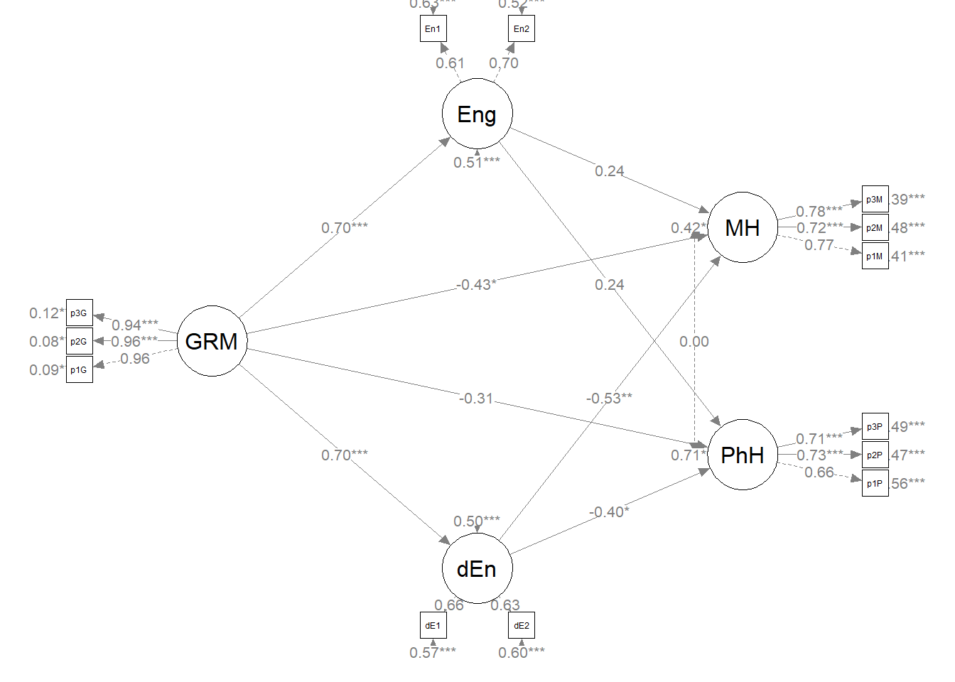
Our global fit indices were strong, \(\chi^2(59) = 59.999, p = 0.439, CFI = 0.999, RMSEA = 0.009, 90CI[0.000, 0.042], SRMR = 0.043\). Yet the indirect effects for engagement remained non-significant. When mental health was the dependent variable, \(B = 0.145, p = 0.098\); when physical health was the dependent variable, \(B = 0.140, p = 0.152\).
If we formally compare the results, we can only use the AIC and BIC with lower values indicating better fit.
## Warning in lavaan::lavTestLRT(struct_fit1, struct_fit4): lavaan WARNING: some
## models are based on a different set of observed variables
##
## Chi-Squared Difference Test
##
## Df AIC BIC Chisq Chisq diff RMSEA Df diff Pr(>Chisq)
## struct_fit4 59 5440.6 5595.5 59.999
## struct_fit1 109 6901.7 7111.7 120.324 60.324 0.029898 50 0.1504Remember – ignore the chi-square difference test. These are non-nested models. The AIC and BIC favor our trimmed model.
What would I do? It would be tempting to simply report the results of engagement and disengagement coping – yet the researchers were interested in the potential of all four coping strategies as potential mediators. Because our disengagement coping mediator remained statistically significant throughout all of our exploration, I would probably choose to report the full analysis because it provides useful information to future researchers and practitioners about the important contribution of disengagement coping (while controlling for the other mediators).
11.10.1 APA Style Write-up of the Results
Method/Analytic Strategy
We specified a parallel mediation, predicting mental and physical health directly from gendered racial microaggressions and indirectly through four coping strategies (i.e., spirituality, social support, engagement, disengagement) The primary analysis occurred in two stages. First, we specified and evaluated a measurement model. Data were analyzed with a maximum likelihood approach the package, lavaan (v. 0.6-16).
Results
Preliminary Analyses
- Missing data analyses and managing missing data>
- Bivariate correlations, means, SDs
- Distributional characteristics, assumptions, etc.
- Address limitations and concerns
Primary Analyses Analyzing our proposed multiple mediator model followed the two-step procedure of first establishing a measurement model with acceptable fit to the data and then proceeding to test the structural model. Given that different researchers recommend somewhat differing thresholds to determine the adequacy of fit, We used the following as evidence of good fit: comparative fit indix (CFI) \(\geq 0.95\), root-mean-square error of approximation (RMSEA) \(\leq 0.06\), and the standard root-mean-square residual (SRMR) \(\leq 0.08\). To establish aceptable fit, we used CFI \(\geq 0.90\), RMSEA \(\leq 0.10\), and SRMR \(\leq 0.10\) (Weston & Gore, 2006).
Following recommendations by Little et al. (T. D. Little et al., 2002, 2013), each latent variable with six or more indicators was represented by three parcels. Parcels were created by randomly assigning scale items to the parcels and then calculating the mean, if at least 65% of the items were non-missing. For the four latent variables with only two indicators each, we constrained the factor loadings to be equal. Factor loadings were all strong, statistically significant, and properly valenced. Global fit statistics were within acceptable thresholds (\(\chi^2(102) = 94.122, p = 0.698, CFI = 1.000, RMSEA = 0.000, 90CI[0.000, 0.028], SRMR = 0.034\)). Thus, we proceeded to testing the structural model.
Our structural model was a parallel mediation, predicting mental and physical health directly from gendered racial microaggressions and indirectly through four coping strategies (i.e., spirituality, social support, engagement, disengagement). Results of the global fit indices suggested good fit \(\chi^2(109) = 120.324, p = 0.216, CFI = 0.994, RMSEA = 0.021, 90CI[0.000, 0.041], SRMR = 0.044\). As shown in Table 2 only two of the eight indirect effects was statistically significant. For both, disengagement coping mediated the effect of gendered racial microaggressions on mental health \((B = -0.328, p = 0.007)\) and physical health \((B = -0.241, p = 0.039)\). The model accunted for 48-68% of the variance in the mediators and 58% and 30% of the variance in mental and physical health, respectively.
Although the model fit was strong, we considered respecification. Modification indices suggested adding a path that would result in a serial mediation from gendered racial microaggressions, to spirituality, to social support and then to each of the dependent variables. While model fit \((\chi^2(108) = 111.657, p = 0.385, CFI = 0.998, RMSEA = 0.012, 90CI[0.000, 0.036], SRMR = 0.042)\) was statistically significantly improved in favor of the serially mediated model \((\Delta\chi^2(1) = 8.667, p = 0.032)\), the serially mediated indirect effects to mental \((B = -0.022, p = 0.737)\) and physical health \((B= -0.019, p = 0.800)\) were non-significant. Consequently, we retained our originally hypothesized model.
We also considered model trimming. Considering both theory plus regression weights and associated p values of the originally hypothesized model, we noted that spiritual and social support coping were not statistically significant with low regression weights. We further noted that engagement coping approached statistical significance. We trimmed the spiritual and social support mediators altogether. While the resulting model (with only engagement and disengagement coping) evidenced strong fit \((\chi^2(59) = 59.999, p = 0.439, CFI = 0.999, RMSEA = 0.009, 90CI[0.000, 0.042], SRMR = 0.043)\), the indirect effects to mental health \((B = 0.145, p = 0.098)\) and physical health \((B = 0.140, p = 0.152)\) through engagement coping remained non-significnant. Because conveying information about significant and not signficant paths are important to future researchers and practitioners, we retained the originally hypothesized model.
11.11 STAY TUNED
A section on power analysis is planned and coming soon! My apologies that it’s not quite Ready.
11.12 Practice Problems
In each of these lessons I provide suggestions for practice that allow you to select one or more problems that are graded in difficulty. With each of these options I encourage you to start with a hypothesized model that has at least four variables and is over-identified. Overall you will (a) start with an established measurement model, (b) test a structural model, (c) use modification indices to add a path or covariance and evaluate the change to the model, (d) use strength and significance of regression weights to trim at least one path or covariance and evaluate the change to the model, (e) make a final decision about the model you retain, (f) provide an APA style representation of the results (with table[s] and figure[s]) .
11.12.1 Problem #1: Change the random seed
Simply change the random seed in the data simulation, then rework the problem evaluated in this chapter. It is possible to further simplify this model by deleting a pair of the mediators and/or one of the dependent variables.
11.12.2 Problem #2: Swap one or more of the variables
The Lewis et al. (2017) study included the additional variable of gendered racial identity centrality. Consider substituting it as an independent or dependent variable.
11.12.3 Problem #3: Try something entirely new.
Conduct a hybrid analysis using data for which you have permission and access (e.g., IRB approved data you have collected or from your lab; data you simulate from a published article; data from an open science repository; data from other chapters in this OER).
Regardless of your choic(es) complete all the elements listed in the grading rubric.
Using the lecture and workflow (chart) as a guide, please work through all the steps listed in the proposed assignment/grading rubric.
| Assignment Component | Points Possible | Points Earned |
|---|---|---|
| 1. Identify the structural model you will evaluate. It should have a minimum of four variables and could be one of the prior path-level models you already examined. | 5 | _____ |
| 2. Import the data and format the variables in the model. | 5 | _____ |
| 3. Specify and evaluate a measurement model that you have established. | 10 | _____ |
| 4. Specify and evaluate a structural model. For the purpose of this exercise, the structural model should be over-identified, that is, should have positive degrees of freedom. How many degrees of freedom does your structural model have? | 10 | _____ |
| 5. Use modification indices to add at least one path or covariance. | 10 | _____ |
| 6. Conduct a formal comparison of global fit between the original and respecified model. | 5 | _____ |
| 7. Using the strength and significance of regression weights as a guide, trim at least path or covariance. | 10 | _____ |
| 8. Conduct a formal comparison of global fit between the original (or built) and trimmed model. | 5 | _____ |
| 9. APA style results with table(s) and figure(s). | 5 | _____ |
| 10. Explanation to grader. | 5 | _____ |
| Totals | 65 | _____ |
11.13 Homeworked Example
For more information about the data used in this homeworked example, please refer to the description and codebook located at the end of the introductory lesson in ReCentering Psych Stats. An .rds file which holds the data is located in the Worked Examples folder at the GitHub site the hosts the OER. The file name is ReC.rds.
The suggested practice problem for this chapter is to evaluate the measurement model that would precede the evaluation of a structural model. And actually, we will need to evaluate two measurement models – an “all items” on indicators model and a parceled model.
Identify the structural model you will evaluate
It should have a minimum of four variables and could be one of the prior path-level models you already examined.
X = Centering: explicit recentering (0 = precentered; 1 = recentered) M1 = TradPed: traditional pedagogy (continuously scaled with higher scores being more favorable) M2 = SRPed: socially responsive pedagogy (continuously scaled with higher scores being more favorable) Y = Valued: valued by me (continuously scaled with higher scores being more favorable)
In this parallel mediation, I am hypothesizing that the perceived course value to the students is predicted by intentional recentering through their assessments of traditional and socially responsive pedagogy.
It helps me to make a quick sketch:
Import the data and format the variables in the model.
The approach we are taking to complex mediation does not allow dependency in the data. Therefore, we will include only those who took the multivariate class (i.e., excluding responses for the ANOVA and psychometrics courses).
Although this dataset is overall small, I will go ahead and make a babydf with the item-level variables.
babydf <- dplyr::select(raw, Centering, ClearResponsibilities, EffectiveAnswers,
    Feedback, ClearOrganization, ClearPresentation, ValObjectives, IncrUnderstanding,
    IncrInterest, InclusvClassrm, EquitableEval, MultPerspectives, DEIintegration)
Let’s check the structure of the variables:
## Classes 'data.table' and 'data.frame':   84 obs. of  13 variables:
##  $ Centering            : Factor w/ 2 levels "Pre","Re": 2 2 2 2 2 2 2 2 2 2 ...
##  $ ClearResponsibilities: int  4 5 5 5 4 3 5 5 3 5 ...
##  $ EffectiveAnswers     : int  4 5 5 4 4 3 5 5 4 4 ...
##  $ Feedback             : int  4 5 4 4 5 4 5 4 4 5 ...
##  $ ClearOrganization    : int  3 5 5 4 4 3 5 5 4 5 ...
##  $ ClearPresentation    : int  4 5 5 3 4 2 5 4 5 5 ...
##  $ ValObjectives        : int  5 5 5 4 4 5 5 4 4 5 ...
##  $ IncrUnderstanding    : int  4 5 5 3 4 3 5 4 5 5 ...
##  $ IncrInterest         : int  4 5 4 3 4 3 5 4 5 4 ...
##  $ InclusvClassrm       : int  5 5 5 5 5 4 5 5 5 5 ...
##  $ EquitableEval        : int  4 5 5 5 4 4 5 4 5 5 ...
##  $ MultPerspectives     : int  4 5 5 5 5 5 5 4 5 5 ...
##  $ DEIintegration       : int  5 5 5 5 5 5 5 5 5 5 ...
##  - attr(*, ".internal.selfref")=<externalptr>
All of the item-level variables are integers (i.e., numerical). This is fine.
The centering variable will need to be dummy coded as 0/1:
## Classes 'data.table' and 'data.frame':   84 obs. of  14 variables:
##  $ Centering            : Factor w/ 2 levels "Pre","Re": 2 2 2 2 2 2 2 2 2 2 ...
##  $ ClearResponsibilities: int  4 5 5 5 4 3 5 5 3 5 ...
##  $ EffectiveAnswers     : int  4 5 5 4 4 3 5 5 4 4 ...
##  $ Feedback             : int  4 5 4 4 5 4 5 4 4 5 ...
##  $ ClearOrganization    : int  3 5 5 4 4 3 5 5 4 5 ...
##  $ ClearPresentation    : int  4 5 5 3 4 2 5 4 5 5 ...
##  $ ValObjectives        : int  5 5 5 4 4 5 5 4 4 5 ...
##  $ IncrUnderstanding    : int  4 5 5 3 4 3 5 4 5 5 ...
##  $ IncrInterest         : int  4 5 4 3 4 3 5 4 5 4 ...
##  $ InclusvClassrm       : int  5 5 5 5 5 4 5 5 5 5 ...
##  $ EquitableEval        : int  4 5 5 5 4 4 5 4 5 5 ...
##  $ MultPerspectives     : int  4 5 5 5 5 5 5 4 5 5 ...
##  $ DEIintegration       : int  5 5 5 5 5 5 5 5 5 5 ...
##  $ CEN                  : num  1 1 1 1 1 1 1 1 1 1 ...
##  - attr(*, ".internal.selfref")=<externalptr>
Specify and evaluate a measurement model that you have established.
As noted in the homeworked example establishing a measurement model for this dataset may seem tricky. That is, with five, four, and three items on each of the constructs, it seems odd to parcel. Previous researchers have parceled scales that have more than three items, even when some parcels will have one item each (Spengler et al., 2023). Correspondingly, I will randomly assign the scales with more than three items each to three parcels.
Here I assign the TradPed items to the 3 parcels.
set.seed(230916)
items <- c("ClearResponsibilities", "EffectiveAnswers", "Feedback", "ClearOrganization",
    "ClearPresentation")
parcels <- c("p1_TR", "p2_TR", "p3_TR")
data.frame(items = sample(items), parcel = rep(parcels, length = length(items)))
## items parcel
## 1 ClearPresentation p1_TR
## 2 Feedback p2_TR
## 3 ClearResponsibilities p3_TR
## 4 EffectiveAnswers p1_TR
## 5 ClearOrganization p2_TRI can now create the parcels using the traditional scoring procedure. Given that we will allow single-item representations, I will sore the 2-item variables if at least one is present (i.e., .5).
As a variable, ClearResponsibilities will stand alone (i.e., the scoring mechanism won’t work on a single variable). Therefore, I will
TRp1_vars <- c("ClearPresentation", "EffectiveAnswers")
TRp2_vars <- c("Feedback", "ClearOrganization")

babydf$p1T <- sjstats::mean_n(babydf[, ..TRp1_vars], 0.5)
babydf$p2T <- sjstats::mean_n(babydf[, ..TRp2_vars], 0.5)

# for consistency, I will create a third parcel from the
# ClearResponsibilities variable by duplicating and renaming it

babydf$p3T <- babydf$ClearResponsibilities

# If the scoring code above does not work for you, try the format
# below which involves removing the periods in front of the variable
# list. One example is provided. babydf$p2T <-
# sjstats::mean_n(babydf[, TRp1_vars], .5)
Here I assign the socially responsive pedagogy items to three parcels.
set.seed(230916)
items <- c("InclusvClassrm", "EquitableEval", "MultPerspectives", "DEIintegration")
parcels <- c("p1_SR", "p2_SR", "p3_SR")
data.frame(items = sample(items), parcel = rep(parcels, length = length(items)))
## items parcel
## 1 InclusvClassrm p1_SR
## 2 MultPerspectives p2_SR
## 3 DEIintegration p3_SR
## 4 EquitableEval p1_SROnly parcel one needs to be scored; the remaining are the single items.
SRp1_vars <- c("InclusvClassrm", "EquitableEval")

babydf$p1S <- sjstats::mean_n(babydf[, ..SRp1_vars], 0.5)

# Here I create the second and third parcels from the individual
# items by duplicating and naming them

babydf$p2S <- babydf$MultPerspectives
babydf$p3S <- babydf$DEIintegration

# If the scoring code above does not work for you, try the format
# below which involves removing the periods in front of the variable
# list. One example is provided. babydf$p1S <-
# sjstats::mean_n(babydf[, SRp1_vars], .5)
I will create “parcels” for the three valued items by naming and duplicating.
babydf$p1V <- babydf$ValObjectives
babydf$p2V <- babydf$IncrUnderstanding
babydf$p3V <- babydf$IncrInterest
msmt_mod <- "
##measurement model
CTR =~ CEN #this is a single item indicator, I had to add code below to set the variance
TrP =~ p1T + p2T + p3T
SRP =~ p1S + p2S + p3S
Val =~ p1V + p2V + p3V
# Variance of the single item indicator
CTR ~~ 0*CEN
# Covariances
CTR ~~ TrP
CTR ~~ SRP
CTR ~~ Val
TrP ~~ SRP
TrP ~~ Val
SRP ~~ Val
"
set.seed(230916)
msmt_fit <- lavaan::cfa(msmt_mod, data = babydf, missing = "fiml")
msmt_fit_sum <- lavaan::summary(msmt_fit, fit.measures = TRUE, standardized = TRUE)
msmt_fit_sum## lavaan 0.6.17 ended normally after 82 iterations
##
## Estimator ML
## Optimization method NLMINB
## Number of model parameters 35
##
## Number of observations 84
## Number of missing patterns 5
##
## Model Test User Model:
##
## Test statistic 51.639
## Degrees of freedom 30
## P-value (Chi-square) 0.008
##
## Model Test Baseline Model:
##
## Test statistic 561.645
## Degrees of freedom 45
## P-value 0.000
##
## User Model versus Baseline Model:
##
## Comparative Fit Index (CFI) 0.958
## Tucker-Lewis Index (TLI) 0.937
##
## Robust Comparative Fit Index (CFI) 0.951
## Robust Tucker-Lewis Index (TLI) 0.927
##
## Loglikelihood and Information Criteria:
##
## Loglikelihood user model (H0) -635.472
## Loglikelihood unrestricted model (H1) -609.652
##
## Akaike (AIC) 1340.943
## Bayesian (BIC) 1426.022
## Sample-size adjusted Bayesian (SABIC) 1315.614
##
## Root Mean Square Error of Approximation:
##
## RMSEA 0.093
## 90 Percent confidence interval - lower 0.047
## 90 Percent confidence interval - upper 0.134
## P-value H_0: RMSEA <= 0.050 0.060
## P-value H_0: RMSEA >= 0.080 0.709
##
## Robust RMSEA 0.103
## 90 Percent confidence interval - lower 0.058
## 90 Percent confidence interval - upper 0.146
## P-value H_0: Robust RMSEA <= 0.050 0.030
## P-value H_0: Robust RMSEA >= 0.080 0.821
##
## Standardized Root Mean Square Residual:
##
## SRMR 0.052
##
## Parameter Estimates:
##
## Standard errors Standard
## Information Observed
## Observed information based on Hessian
##
## Latent Variables:
## Estimate Std.Err z-value P(>|z|) Std.lv Std.all
## CTR =~
## CEN 1.000 0.483 1.000
## TrP =~
## p1T 1.000 0.691 0.912
## p2T 0.963 0.090 10.727 0.000 0.666 0.850
## p3T 0.952 0.108 8.848 0.000 0.658 0.757
## SRP =~
## p1S 1.000 0.497 0.936
## p2S 1.061 0.134 7.944 0.000 0.527 0.761
## p3S 1.408 0.179 7.852 0.000 0.700 0.807
## Val =~
## p1V 1.000 0.352 0.562
## p2V 2.238 0.399 5.608 0.000 0.788 0.925
## p3V 2.200 0.400 5.495 0.000 0.774 0.852
##
## Covariances:
## Estimate Std.Err z-value P(>|z|) Std.lv Std.all
## CTR ~~
## .CEN 0.000 0.000 NaN
## TrP 0.075 0.039 1.907 0.056 0.225 0.225
## SRP 0.068 0.029 2.357 0.018 0.283 0.283
## Val 0.032 0.021 1.539 0.124 0.187 0.187
## TrP ~~
## SRP 0.273 0.053 5.122 0.000 0.795 0.795
## Val 0.219 0.053 4.132 0.000 0.902 0.902
## SRP ~~
## Val 0.121 0.032 3.783 0.000 0.691 0.691
##
## Intercepts:
## Estimate Std.Err z-value P(>|z|) Std.lv Std.all
## .CEN 0.369 0.053 7.009 0.000 0.369 0.765
## .p1T 4.321 0.083 52.220 0.000 4.321 5.698
## .p2T 4.196 0.085 49.115 0.000 4.196 5.359
## .p3T 4.478 0.095 47.081 0.000 4.478 5.152
## .p1S 4.637 0.058 80.049 0.000 4.637 8.734
## .p2S 4.411 0.076 58.169 0.000 4.411 6.367
## .p3S 4.360 0.099 43.986 0.000 4.360 5.029
## .p1V 4.464 0.068 65.385 0.000 4.464 7.134
## .p2V 4.190 0.093 45.087 0.000 4.190 4.919
## .p3V 3.986 0.099 40.142 0.000 3.986 4.389
##
## Variances:
## Estimate Std.Err z-value P(>|z|) Std.lv Std.all
## .CEN 0.000 0.000 0.000
## .p1T 0.097 0.026 3.798 0.000 0.097 0.169
## .p2T 0.170 0.035 4.918 0.000 0.170 0.277
## .p3T 0.322 0.057 5.689 0.000 0.322 0.427
## .p1S 0.035 0.019 1.878 0.060 0.035 0.124
## .p2S 0.202 0.040 5.075 0.000 0.202 0.421
## .p3S 0.262 0.056 4.714 0.000 0.262 0.349
## .p1V 0.268 0.043 6.199 0.000 0.268 0.684
## .p2V 0.105 0.036 2.966 0.003 0.105 0.145
## .p3V 0.226 0.048 4.744 0.000 0.226 0.274
## CTR 0.233 0.036 6.481 0.000 1.000 1.000
## TrP 0.478 0.090 5.316 0.000 1.000 1.000
## SRP 0.247 0.047 5.291 0.000 1.000 1.000
## Val 0.124 0.046 2.700 0.007 1.000 1.000msmt_fit_pEsts <- lavaan::parameterEstimates(msmt_fit, boot.ci.type = "bca.simple",
standardized = TRUE)
# msmt_fit_pEsts #To reduce redundancy in the book, I did not print
# the parameter estimates. Their object is used in exporting a .csv
# file.Below is script that will export the global fit indices (via tidySEM::table_fit) and the parameter estimates (e.g., factor loadings, structural regression weights, and parameters we requested such as the indirect effect) to .csv files that you can manipulate outside of R.
# global fit indices
msmt_globalfit <- tidySEM::table_fit(msmt_fit)
write.csv(msmt_globalfit, file = "msmt_globalfit.csv")
# the code below writes the parameter estimates into a .csv file
write.csv(msmt_fit_pEsts, file = "msmt_fit_pEsts.csv")
Here is how I wrote up the results:
Analyzing our proposed parallel mediation followed the two-step procedure of first establishing a measurement model with acceptable fit to the data and then proceeding to test the structural model. Given that different researchers recommend somewhat differing thresholds to determine the adequacy of fit, We used the following as evidence of good fit: comparative fit indix (CFI) \(\geq 0.95\), root-mean-square error of approximation (RMSEA) \(\leq 0.06\), and the standard root-mean-square residual (SRMR) \(\leq 0.08\). To establish aceptable fit, we used CFI \(\geq 0.90\), RMSEA \(\leq 0.10\), and SRMR \(\leq 0.10\) (Weston & Gore, 2006).
We evaluated the measurement model by following recommendations by Little et al. (T. D. Little et al., 2002, 2013). The three course evaluation scales representing traditional pedagogy (5 items), socially responsive pedagogy (4 items), and perceived value to the student (3) were each represented by a combination of parcels and single items that created just-identified factors (i.e., the five items of traditional pedagogy were randomly assigned across three parcels and mean scores were used). For the centering variable – a single item indicator – we constrained the variance to zero.
With the exception of the statistically significant chi-square, fit statistics evidenced a mix of good and acceptable thresholds \((\chi^2(30) = 51.639, p = 0.004, CFI = 0.958, RMSEA = 0.093, 90CI[0.047, 0.134], SRMR = 0.052)\). Thus, we proceeded to testing the structural model. The strong, statistically significant, and properly valanced factor loadings are presented in Table 1.
Table 1
|Factor Loadings for the Measurement Model
|:————————————————————-|
| Latent variable and indicator | est | SE | p | est_std |
| Traditional Pedagogy | ||||
| Parcel 1 | 1.000 | 0.000 | 0.912 | |
| Parcel 2 | 0.963 | 0.090 | <0.001 | 0.850 |
| Parcel 3 | 0.952 | 0.108 | <0.001 | 0.757 |
| Socially Responsive Pedagogy | ||||
| Parcel 1 | 1.000 | 0.000 | 0.936 | |
| Parcel 2 | 1.061 | 0.134 | <0.001 | 0.761 |
| Parcel 3 | 1.408 | 0.179 | <0.001 | 0.807 |
| Perceived Value to the Student | ||||
| Item 1 | 1.000 | 0.000 | 0.562 | |
| Item 2 | 2.238 | 0.399 | <0.001 | 0.925 |
| Item 3 | 2.200 | 0.400 | <0.001 | 0.852 |
| CENTERING | 1.000 | 0.000 | 1.000 |
Although it likely would not appear in an article (no space), here is a figure of my measurement model. We can use it to clarify our conceptual understanding of what we specified and check our work.
semPlot::semPaths(msmt_fit, what = "col", whatLabels = "stand", sizeMan = 5,
    node.width = 1, edge.label.cex = 0.75, style = "lisrel", mar = c(2,
        2, 2, 2))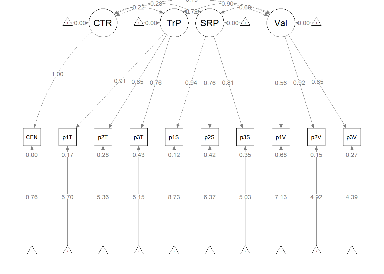
Specify and evaluate a structural model
As a reminder, I am hypothesizing a parallel mediation where the perceived course value to the students is predicted by intentional recentering through their assessments of traditional and socially responsive pedagogy.
X = Centering: explicit recentering (0 = precentered; 1 = recentered) M1 = TradPed: traditional pedagogy (continuously scaled with higher scores being more favorable) M2 = SRPed: socially responsive pedagogy (continuously scaled with higher scores being more favorable) Y = Valued: valued by me (continuously scaled with higher scores being more favorable)
For the purpose of this exercise, the structural model should be over-identified, that is, should have positive degrees of freedom. How many degrees of freedom does your structural model have?
**Knowns::: \(\frac{k(k+1)}{2}\) where k is the number of constructs
## [1] 10There are 10 knowns.
Unknowns:
- Exogenous (predictor) variables (1 variance estimated for each): we have 1 (CTR)
- Endogenous (predicted) variables (1 disturbance variance for each): we have 3 (TrP, SRP, Val)
- Correlations between variables (1 covariance for each pairing): we have 0
- Regression paths (arrows linking exogenous variables to endogenous variables): we have 5
With 10 knowns and 9 unknowns, we have 1 degree of freedom in the structural portion of the model. This is an over-identified model.
ReC_struct_mod1 <- "
        #measurement model
         CTR =~ CEN #this is a single item indicator, I had to add code below to set the variance
         TrP =~ p1T + p2T + p3T
         SRP =~ p1S + p2S + p3S
         Val =~ p1V + p2V + p3V

        # Variance of the single item indicator
         CTR ~~ 0*CEN

        #structural model
          Val ~ b1*TrP + b2*SRP + c_p*CTR
          TrP ~ a1*CTR
          SRP ~ a2*CTR

          indirect1 := a1 * b1
          indirect2 := a2 * b2
          contrast := indirect1 - indirect2
          total_indirects := indirect1 + indirect2
          total_c    := c_p + (indirect1) + (indirect2)
          direct := c_p

          "
set.seed(230916)  #needed for reproducibility especially when specifying bootstrapped confidence intervals
ReC_struct_fit1 <- lavaan::sem(ReC_struct_mod1, data = babydf, missing = "fiml",
    fixed.x = FALSE)
ReC_struct_summary1 <- lavaan::summary(ReC_struct_fit1, fit.measures = TRUE,
    standardized = TRUE, rsq = TRUE)
ReC_struct_pEsts1 <- lavaan::parameterEstimates(ReC_struct_fit1, boot.ci.type = "bca.simple",
    standardized = TRUE)
ReC_struct_summary1
## lavaan 0.6.17 ended normally after 72 iterations
##
## Estimator ML
## Optimization method NLMINB
## Number of model parameters 34
##
## Number of observations 84
## Number of missing patterns 5
##
## Model Test User Model:
##
## Test statistic 105.390
## Degrees of freedom 31
## P-value (Chi-square) 0.000
##
## Model Test Baseline Model:
##
## Test statistic 561.645
## Degrees of freedom 45
## P-value 0.000
##
## User Model versus Baseline Model:
##
## Comparative Fit Index (CFI) 0.856
## Tucker-Lewis Index (TLI) 0.791
##
## Robust Comparative Fit Index (CFI) 0.858
## Robust Tucker-Lewis Index (TLI) 0.794
##
## Loglikelihood and Information Criteria:
##
## Loglikelihood user model (H0) -662.347
## Loglikelihood unrestricted model (H1) -609.652
##
## Akaike (AIC) 1392.694
## Bayesian (BIC) 1475.342
## Sample-size adjusted Bayesian (SABIC) 1368.088
##
## Root Mean Square Error of Approximation:
##
## RMSEA 0.169
## 90 Percent confidence interval - lower 0.134
## 90 Percent confidence interval - upper 0.205
## P-value H_0: RMSEA <= 0.050 0.000
## P-value H_0: RMSEA >= 0.080 1.000
##
## Robust RMSEA 0.173
## 90 Percent confidence interval - lower 0.136
## 90 Percent confidence interval - upper 0.210
## P-value H_0: Robust RMSEA <= 0.050 0.000
## P-value H_0: Robust RMSEA >= 0.080 1.000
##
## Standardized Root Mean Square Residual:
##
## SRMR 0.226
##
## Parameter Estimates:
##
## Standard errors Standard
## Information Observed
## Observed information based on Hessian
##
## Latent Variables:
## Estimate Std.Err z-value P(>|z|) Std.lv Std.all
## CTR =~
## CEN 1.000 0.483 1.000
## TrP =~
## p1T 1.000 0.675 0.891
## p2T 1.012 0.100 10.149 0.000 0.684 0.873
## p3T 0.974 0.115 8.448 0.000 0.658 0.757
## SRP =~
## p1S 1.000 0.467 0.879
## p2S 1.160 0.148 7.851 0.000 0.541 0.780
## p3S 1.595 0.205 7.798 0.000 0.744 0.863
## Val =~
## p1V 1.000 0.335 0.544
## p2V 2.220 0.394 5.633 0.000 0.743 0.913
## p3V 2.197 0.398 5.527 0.000 0.736 0.842
##
## Regressions:
## Estimate Std.Err z-value P(>|z|) Std.lv Std.all
## Val ~
## TrP (b1) 0.439 0.092 4.763 0.000 0.885 0.885
## SRP (b2) 0.087 0.079 1.091 0.275 0.121 0.121
## CTR (c_p) -0.029 0.053 -0.543 0.587 -0.042 -0.042
## TrP ~
## CTR (a1) 0.319 0.158 2.017 0.044 0.228 0.228
## SRP ~
## CTR (a2) 0.311 0.109 2.865 0.004 0.321 0.321
##
## Covariances:
## Estimate Std.Err z-value P(>|z|) Std.lv Std.all
## CTR ~~
## .CEN 0.000 0.000 NaN
##
## Intercepts:
## Estimate Std.Err z-value P(>|z|) Std.lv Std.all
## .CEN 0.369 0.053 7.009 0.000 0.369 0.765
## .p1T 4.321 0.083 52.220 0.000 4.321 5.698
## .p2T 4.196 0.085 49.115 0.000 4.196 5.359
## .p3T 4.478 0.095 47.068 0.000 4.478 5.151
## .p1S 4.637 0.058 80.049 0.000 4.637 8.734
## .p2S 4.413 0.076 58.132 0.000 4.413 6.363
## .p3S 4.359 0.098 44.348 0.000 4.359 5.051
## .p1V 4.464 0.067 66.486 0.000 4.464 7.254
## .p2V 4.190 0.089 47.193 0.000 4.190 5.149
## .p3V 3.986 0.096 41.739 0.000 3.986 4.564
##
## Variances:
## Estimate Std.Err z-value P(>|z|) Std.lv Std.all
## .CEN 0.000 0.000 0.000
## .p1T 0.119 0.032 3.701 0.000 0.119 0.207
## .p2T 0.146 0.036 4.075 0.000 0.146 0.237
## .p3T 0.323 0.058 5.539 0.000 0.323 0.427
## .p1S 0.064 0.022 2.961 0.003 0.064 0.227
## .p2S 0.188 0.039 4.816 0.000 0.188 0.391
## .p3S 0.191 0.057 3.321 0.001 0.191 0.256
## .p1V 0.267 0.043 6.193 0.000 0.267 0.704
## .p2V 0.110 0.036 3.076 0.002 0.110 0.166
## .p3V 0.222 0.047 4.682 0.000 0.222 0.290
## CTR 0.233 0.036 6.481 0.000 1.000 1.000
## .TrP 0.432 0.087 4.992 0.000 0.948 0.948
## .SRP 0.195 0.043 4.498 0.000 0.897 0.897
## .Val 0.023 0.011 2.141 0.032 0.205 0.205
##
## R-Square:
## Estimate
## CEN 1.000
## p1T 0.793
## p2T 0.763
## p3T 0.573
## p1S 0.773
## p2S 0.609
## p3S 0.744
## p1V 0.296
## p2V 0.834
## p3V 0.710
## TrP 0.052
## SRP 0.103
## Val 0.795
##
## Defined Parameters:
## Estimate Std.Err z-value P(>|z|) Std.lv Std.all
## indirect1 0.140 0.075 1.869 0.062 0.202 0.202
## indirect2 0.027 0.026 1.023 0.306 0.039 0.039
## contrast 0.113 0.082 1.386 0.166 0.163 0.163
## total_indircts 0.167 0.077 2.163 0.031 0.241 0.241
## total_c 0.138 0.083 1.670 0.095 0.199 0.199
## direct -0.029 0.053 -0.543 0.587 -0.042 -0.042# ReC_struct_pEsts1 #although creating the object is useful to export
# as a .csv I didn't ask it to print into the book\((\chi^2(31) = 105.390, p < 0.001, CFI = 0.856, RMSEA = 0.169, 90CI[0.134, 0.205], SRMR = 0.226)\).
Below is script that will export the global fit indices (via tidySEM::table_fit) and the parameter estimates (e.g., factor loadings, structural regression weights, and parameters we requested such as the indirect effect) to .csv files that you can manipulate outside of R.
# global fit indices
ReC_globalfit1 <- tidySEM::table_fit(ReC_struct_fit1)
write.csv(ReC_globalfit1, file = "ReC_globalfit1.csv")
# the code below writes the parameter estimates into a .csv file
write.csv(ReC_struct_pEsts1, file = "ReC_struct_pEsts1.csv")
Let’s work up a figure
plot_ReC_struct1 <- semPlot::semPaths(ReC_struct_fit1, what = "col", whatLabels = "stand",
    sizeMan = 3, node.width = 1, edge.label.cex = 0.75, style = "lisrel",
    mar = c(2, 2, 2, 2), structural = FALSE, curve = FALSE, intercepts = FALSE)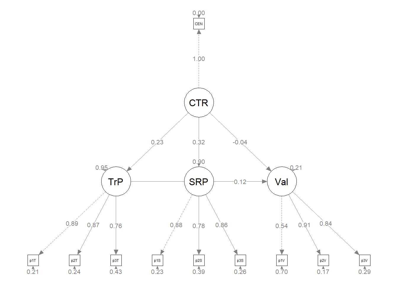
| Grid for Plotting semplot::sempath | ||
|---|---|---|
| (1,1) empty | (1,2) TrP | (1,3) empty |
| (2,1) CTR | (2,2) empty | (2,3) Val |
| (3,1) empty | (3,2) SRP | (3,3) empty |
We place these values along with the names of our latent variables in to the semptools::layout_matrix function.
# IMPORTANT: Must use the node names (take directly from the SemPlot)
# assigned by SemPlot You can change them as the last thing
m1_msmt <- semptools::layout_matrix(CTR = c(2, 1), TrP = c(1, 2), SRP = c(3,
    2), Val = c(2, 3))
Next we provide instruction on the direction (up, down, left, right) we want the indicator/observed variables to face. We identify the direction by the location of each of our latent variables. For example, in the code below we want the indicators for the REM variable (2,1) to face left.
# tell where you want the indicators to face
m1_point_to <- semptools::layout_matrix(left = c(2, 1), up = c(1, 2), down = c(3,
    2), right = c(2, 3))
The next two sets of code work together to specify the order of the observed variables for each factor. in the top set of code the variable names indicate the order in which they will appear (i.e., p1R, p2R, p3R). In the second set of code, the listing the variable name three times (i.e., REM, REM, REM) serves as a placeholder for each of the indicators.
It is critical to note that we need to use the abbreviated variable names assigned by semTools::semPaths and not necessarily the names that are in the dataframe.
# the next two codes -- indicator_order and indicator_factor are
# paired together, they specify the order of observed variables for
# each factor
m1_indicator_order <- c("CEN", "p1T", "p2T", "p3T", "p1S", "p2S", "p3S",
    "p1V", "p2V", "p3V")

m1_indicator_factor <- c("CTR", "TrP", "TrP", "TrP", "SRP", "SRP", "SRP",
    "Val", "Val", "Val")
The next two sets of codes provide some guidance about how far away the indicator (square/rectangular) variables should be away from the latent (oval/circular) variables. Subsequently, the next set of values indicate how far away each of the indicator (square/rectangular) variables should be spread apart.
# next set of code pushes the indicator variables away from the
# factor
m1_indicator_push <- c(CTR = 1, TrP = 1, SRP = 1, Val = 1)


# spreading the boxes away from each other
m1_indicator_spread <- c(CTR = 0.5, TrP = 2.5, SRP = 2.5, Val = 1)
Finally, we can feed all of the objects that whole these instructions into the semptools::sem_set_layout function. If desired, we can use the semptools::change_node_label function to rename the latent variables. Again, make sure to use the variable names that semPlot::semPaths has assigned.
plot1 <- semptools::set_sem_layout(plot_ReC_struct1, indicator_order = m1_indicator_order,
    indicator_factor = m1_indicator_factor, factor_layout = m1_msmt, factor_point_to = m1_point_to,
    indicator_push = m1_indicator_push, indicator_spread = m1_indicator_spread)

# changing node labels plot1 <- semptools::change_node_label(plot1,
# c(CTR = 'CTRing', TrP = 'TradPed', SRP = 'SRPed', Val = 'Valued'),
# label.cex = 1.1)

# adding stars to indicate significant paths
plot1 <- semptools::mark_sig(plot1, ReC_struct_fit1)

plot(plot1)
If we table the results, here’s what we have:
Table 2
| Model Coefficients Assessing the Effect of Perceived Value from Recentering through Socially Responsive and Traditional Pedagogies |
|---|
| Predictor | \(B\) | \(SE_{B}\) | \(p\) | \(\beta\) | \(R^2\) |
|---|---|---|---|---|---|
| Traditional Pedagogy (M1) | .05 | ||||
| Centering (\(a_1\)) | 0.319 | 0.158 | 0.044 | 0.228 | |
| Socially Responsive Pedagogy (M2) | .10 | ||||
| Centering (\(a_2\)) | 0.311 | 0.109 | 0.004 | 0.321 | |
| Perceived Value (DV) | .80 | ||||
| Traditional Pedagogy (\(b_1\)) | 0.595 | 0.050 | 0.000 | 0.865 | |
| Socially Responsive Pedagogy (\(b_2\)) | 0.087 | 0.079 | 0.275 | 0.121 | |
| Centering (\(c'\)) | -0.029 | 0.053 | 0.587 | -0.042 |
| Effects | \(B\) | \(SE_{B}\) | \(p\) | 95% CI | |
|---|---|---|---|---|---|
| Indirect(\(a_1*b_1\)) | 0.140 | 0.075 | 0.062 | 0.202 | -0.007, 0.287 |
| Indirect(\(a_2*b_2\)) | 0.027 | 0.026 | 0.306 | 0.039 | -0.025, 0.078 |
| Contrast | 0.113 | 0.082 | 0.166 | 0.163 | -0.047, 0.273 |
| Total indirects | 0.167 | 0.077 | 0.031 | 0.241 | 0.016, 0.318 |
| Total effect | 0.138 | 0.083 | 0.095 | 0.199 | -0.024, 0.300 |
| Note. The significance of the indirect effects was calculated with bootstrapped, bias-corrected, confidence intervals (.95). |
Our structural model was a parallel mediation, predicting perceived value to the student directly from centering and indirectly through traditional and socially responsive pedagogy. Results of the global fit indices all fell below the thresholds of acceptability \((\chi^2(31) = 105.390, p < 0.001, CFI = 0.856, RMSEA = 0.169, 90CI[0.134, 0.205, SRMR = 0.226)\). As shown in Table 2, although the model accounted for 95% of the variance in perceived value, neither of the indirect effects were statistically significant. Only traditional and socially responsive pedagogy appeared to have significant influence on perceived value. Thus, we considered the possibility of forward searching to build the model.
Use modification indices to add at least one path or covariance
Normally, we would use the lavaan::modindices() function to retrieve the modification indices. Unfortunately, it is not working and I cannot understand why. This error does not make sense to me. I wonder if this error and the inability to plot the result is related to the dichotomous predictor variable? Who knows. If anyone discovers a solution, please let me know!
I planned this problem knowing that the the only logical path would be to add a path from traditional pedagogy to socially responsive pedagogy, turning this into a serial mediation. Let’s do that!
Before even conducting the statistic, adding this path will make the structural model just-identified. As such, it will have the identical strong fit of the measurement model. This means we probably should not favor this model if the serial indirect effect is not statistically significant.
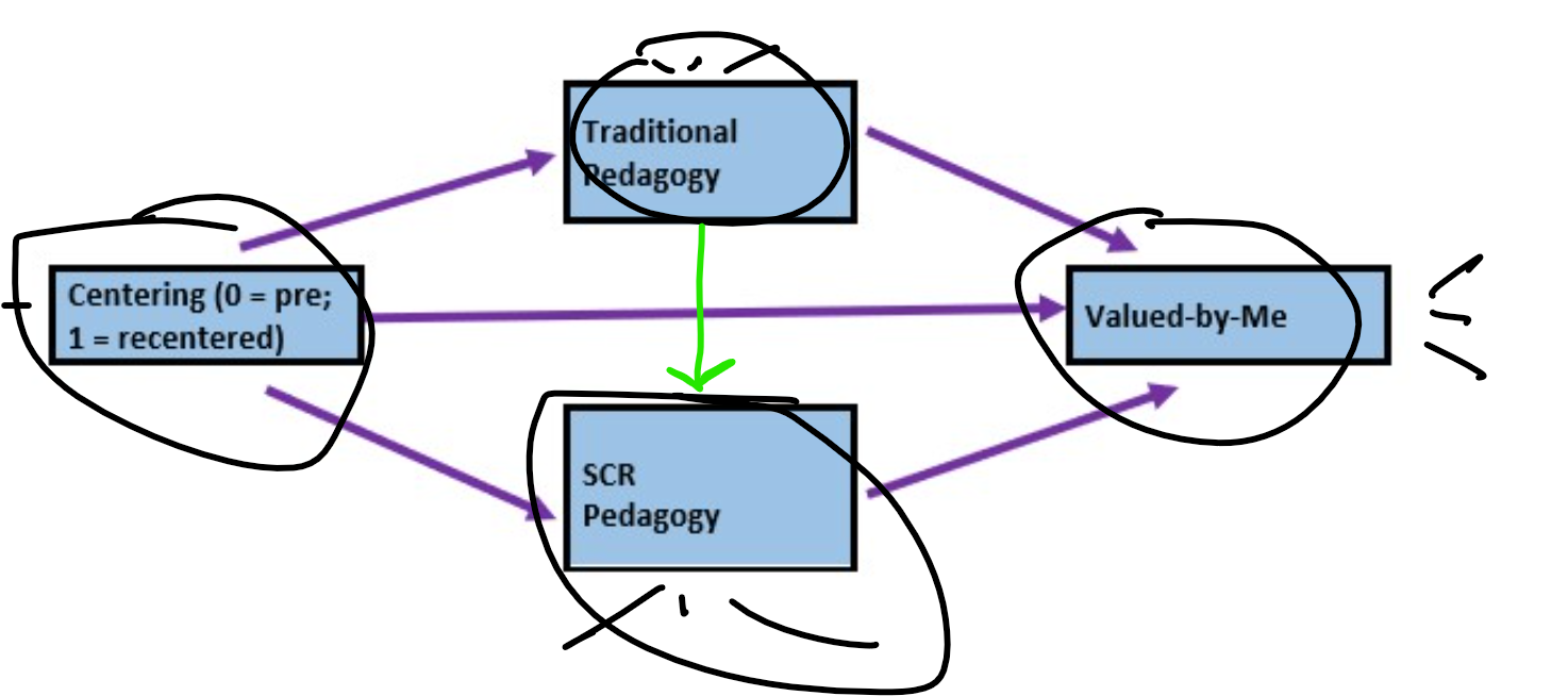
Conduct a formal comparison of global fit between the original and respecified model
ReC_struct_mod2 <- "
        #measurement model
         CTR =~ CEN #this is a single item indicator, I had to add code below to set the variance
         TrP =~ p1T + p2T + p3T
         SRP =~ p1S + p2S + p3S
         Val =~ p1V + p2V + p3V

        # Variance of the single item indicator
         CTR ~~ 0*CEN

        #structural model
          Val ~ b1*TrP + b2*SRP + c_p*CTR
          TrP ~ a1*CTR
          SRP ~ a2*CTR + d1*TrP


          indirect1 := a1 * b1
          indirect2 := a2 * b2
          indirect3 := a1 * d1 * b2
          contrast1 := indirect1 - indirect2
          contrast2 := indirect1 - indirect3
          contrast3 := indirect2 - indirect3
          total_indirects := indirect1 + indirect2 + indirect3
          total_c    := c_p + (indirect1) + (indirect2) + (indirect3)
          direct := c_p

          "
set.seed(230916)  #needed for reproducibility especially when specifying bootstrapped confidence intervals
ReC_struct_fit2 <- lavaan::sem(ReC_struct_mod2, data = babydf, missing = "fiml")
ReC_struct_summary2 <- lavaan::summary(ReC_struct_fit2, fit.measures = TRUE,
    standardized = TRUE, rsq = TRUE)
ReC_struct_pEsts2 <- lavaan::parameterEstimates(ReC_struct_fit2, boot.ci.type = "bca.simple",
    standardized = TRUE)
ReC_struct_summary2
## lavaan 0.6.17 ended normally after 75 iterations
##
## Estimator ML
## Optimization method NLMINB
## Number of model parameters 35
##
## Number of observations 84
## Number of missing patterns 5
##
## Model Test User Model:
##
## Test statistic 51.639
## Degrees of freedom 30
## P-value (Chi-square) 0.008
##
## Model Test Baseline Model:
##
## Test statistic 561.645
## Degrees of freedom 45
## P-value 0.000
##
## User Model versus Baseline Model:
##
## Comparative Fit Index (CFI) 0.958
## Tucker-Lewis Index (TLI) 0.937
##
## Robust Comparative Fit Index (CFI) 0.951
## Robust Tucker-Lewis Index (TLI) 0.927
##
## Loglikelihood and Information Criteria:
##
## Loglikelihood user model (H0) -635.472
## Loglikelihood unrestricted model (H1) -609.652
##
## Akaike (AIC) 1340.943
## Bayesian (BIC) 1426.022
## Sample-size adjusted Bayesian (SABIC) 1315.614
##
## Root Mean Square Error of Approximation:
##
## RMSEA 0.093
## 90 Percent confidence interval - lower 0.047
## 90 Percent confidence interval - upper 0.134
## P-value H_0: RMSEA <= 0.050 0.060
## P-value H_0: RMSEA >= 0.080 0.709
##
## Robust RMSEA 0.103
## 90 Percent confidence interval - lower 0.058
## 90 Percent confidence interval - upper 0.146
## P-value H_0: Robust RMSEA <= 0.050 0.030
## P-value H_0: Robust RMSEA >= 0.080 0.821
##
## Standardized Root Mean Square Residual:
##
## SRMR 0.052
##
## Parameter Estimates:
##
## Standard errors Standard
## Information Observed
## Observed information based on Hessian
##
## Latent Variables:
## Estimate Std.Err z-value P(>|z|) Std.lv Std.all
## CTR =~
## CEN 1.000 0.483 1.000
## TrP =~
## p1T 1.000 0.691 0.912
## p2T 0.963 0.090 10.727 0.000 0.666 0.850
## p3T 0.952 0.108 8.848 0.000 0.658 0.757
## SRP =~
## p1S 1.000 0.497 0.936
## p2S 1.061 0.134 7.944 0.000 0.527 0.761
## p3S 1.408 0.179 7.852 0.000 0.700 0.807
## Val =~
## p1V 1.000 0.352 0.562
## p2V 2.238 0.399 5.608 0.000 0.788 0.925
## p3V 2.200 0.400 5.495 0.000 0.774 0.852
##
## Regressions:
## Estimate Std.Err z-value P(>|z|) Std.lv Std.all
## Val ~
## TrP (b1) 0.487 0.113 4.308 0.000 0.957 0.957
## SRP (b2) -0.047 0.104 -0.456 0.649 -0.067 -0.067
## CTR (c_p) -0.007 0.053 -0.128 0.898 -0.009 -0.009
## TrP ~
## CTR (a1) 0.322 0.161 1.996 0.046 0.225 0.225
## SRP ~
## CTR (a2) 0.113 0.087 1.291 0.197 0.109 0.109
## TrP (d1) 0.554 0.070 7.963 0.000 0.770 0.770
##
## Covariances:
## Estimate Std.Err z-value P(>|z|) Std.lv Std.all
## CTR ~~
## .CEN 0.000 0.000 NaN
##
## Intercepts:
## Estimate Std.Err z-value P(>|z|) Std.lv Std.all
## .CEN 0.369 0.053 7.009 0.000 0.369 0.765
## .p1T 4.321 0.083 52.220 0.000 4.321 5.698
## .p2T 4.196 0.085 49.115 0.000 4.196 5.359
## .p3T 4.478 0.095 47.081 0.000 4.478 5.152
## .p1S 4.637 0.058 80.049 0.000 4.637 8.734
## .p2S 4.411 0.076 58.169 0.000 4.411 6.367
## .p3S 4.360 0.099 43.986 0.000 4.360 5.029
## .p1V 4.464 0.068 65.385 0.000 4.464 7.134
## .p2V 4.190 0.093 45.087 0.000 4.190 4.919
## .p3V 3.986 0.099 40.142 0.000 3.986 4.389
##
## Variances:
## Estimate Std.Err z-value P(>|z|) Std.lv Std.all
## .CEN 0.000 0.000 0.000
## .p1T 0.097 0.026 3.798 0.000 0.097 0.169
## .p2T 0.170 0.035 4.918 0.000 0.170 0.277
## .p3T 0.322 0.057 5.689 0.000 0.322 0.427
## .p1S 0.035 0.019 1.878 0.060 0.035 0.124
## .p2S 0.202 0.040 5.075 0.000 0.202 0.421
## .p3S 0.262 0.056 4.714 0.000 0.262 0.349
## .p1V 0.268 0.043 6.199 0.000 0.268 0.684
## .p2V 0.105 0.036 2.966 0.003 0.105 0.145
## .p3V 0.226 0.048 4.744 0.000 0.226 0.274
## CTR 0.233 0.036 6.481 0.000 1.000 1.000
## .TrP 0.454 0.086 5.280 0.000 0.949 0.949
## .SRP 0.088 0.023 3.838 0.000 0.357 0.357
## .Val 0.023 0.011 2.087 0.037 0.184 0.184
##
## R-Square:
## Estimate
## CEN 1.000
## p1T 0.831
## p2T 0.723
## p3T 0.573
## p1S 0.876
## p2S 0.579
## p3S 0.651
## p1V 0.316
## p2V 0.855
## p3V 0.726
## TrP 0.051
## SRP 0.643
## Val 0.816
##
## Defined Parameters:
## Estimate Std.Err z-value P(>|z|) Std.lv Std.all
## indirect1 0.157 0.086 1.817 0.069 0.215 0.215
## indirect2 -0.005 0.012 -0.439 0.661 -0.007 -0.007
## indirect3 -0.008 0.019 -0.439 0.661 -0.012 -0.012
## contrast1 0.162 0.090 1.806 0.071 0.223 0.223
## contrast2 0.165 0.097 1.708 0.088 0.227 0.227
## contrast3 0.003 0.010 0.318 0.750 0.004 0.004
## total_indircts 0.143 0.080 1.790 0.073 0.196 0.196
## total_c 0.136 0.086 1.584 0.113 0.187 0.187
## direct -0.007 0.053 -0.128 0.898 -0.009 -0.009# ReC_struct_pEsts1 #although creating the object is useful to export
# as a .csv I didn't ask it to print into the book# global fit indices
ReC_globalfit2 <- tidySEM::table_fit(ReC_struct_fit2)
write.csv(ReC_globalfit2, file = "ReC_globalfit2.csv")
# the code below writes the parameter estimates into a .csv file
write.csv(ReC_struct_pEsts2, file = "ReC_struct_pEsts2.csv")Here is the global fit indices: \((\chi^2(30) = 51.639, p = 0.004, CFI = 0.958, RMSEA = 0.093, 90CI[0.047, 0.134], SRMR = 0.052)\). As I noted before we ran it, they are identical to those of the just-identified measurement model.
We can compare the difference between the originally hypothsized fit and this fit.
##
## Chi-Squared Difference Test
##
##                 Df    AIC    BIC   Chisq Chisq diff   RMSEA Df diff
## ReC_struct_fit2 30 1340.9 1426.0  51.639
## ReC_struct_fit1 31 1392.7 1475.3 105.390     53.751 0.79246       1
##                         Pr(>Chisq)
## ReC_struct_fit2
## ReC_struct_fit1 0.0000000000002276 ***
## ---
## Signif. codes:  0 '***' 0.001 '**' 0.01 '*' 0.05 '.' 0.1 ' ' 1
Given that these models are nested (i.e., same variables, same sample, only the paths change), we can use the \((\Delta\chi^2(1) = 53.751, p < 0.001\) to see that there is a statistically significant difference favoring the model with the serial mediation. If we examine the regression weights and parameters, we see that none of the indirect effects, including the serial mediation \((B = -0.008, SE = 0.019, \beta = -0.012, p = 0.661, 95CI[-0.046, 0.029])\). are non-significant. Thus, I would favor retaining the originally hypothesized model.
plot_struct2 <- semPlot::semPaths(ReC_struct_fit2, what = "col", whatLabels = "stand",
    sizeMan = 3, node.width = 1, edge.label.cex = 0.75, style = "lisrel",
    mar = c(2, 2, 2, 2), structural = FALSE, curve = FALSE, intercepts = FALSE)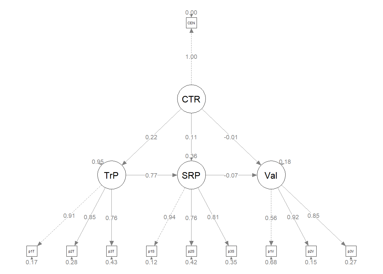
Using the strength and significance of regression weights as a guide, trim at least path or covariance
Given my rejection of the model that resulted from adding the serial mediation, I will inspect the strength, direction, and significance of my regression weights to see about deleting a path.
This is tricky, the “most-nonsignificant” path is the direct path from centering to perceived value \((B = 0.029, p = 0.587)\). That path, however, is involved in the indirect effects (and I would sue like the indirect effect through traditional pedagogy \([B = 0.140, p = 0.061, 95CI(-0.007, 0.287)]\) to pass into statistical significance).The next most non-significant path is \(b_2\), from socially responsive pedagogy to perceived value \((B = 0.087, p = 0.275))\). Let’s trim it.
ReC_struct_mod3 <- "
        #measurement model
         CTR =~ CEN #this is a single item indicator, I had to add code below to set the variance
         TrP =~ p1T + p2T + p3T
         SRP =~ p1S + p2S + p3S
         Val =~ p1V + p2V + p3V

        # Variance of the single item indicator
         CTR ~~ 0*CEN

        #structural model
          Val ~ b1*TrP + c_p*CTR #trimmed + b2*SRP
          TrP ~ a1*CTR
          SRP ~ a2*CTR

          indirect1 := a1 * b1
          #indirect2 := a2 * b2 #trimmed because the b2 path was trimmed
          #contrast := indirect1 - indirect2
          #total_indirects := indirect1 + indirect2
          total_c    := c_p + (indirect1) #trimmed + (indirect2)
          direct := c_p

          "
set.seed(230916)  #needed for reproducibility especially when specifying bootstrapped confidence intervals
ReC_struct_fit3 <- lavaan::sem(ReC_struct_mod3, data = babydf, missing = "fiml",
    fixed.x = FALSE)
ReC_struct_summary3 <- lavaan::summary(ReC_struct_fit3, fit.measures = TRUE,
    standardized = TRUE, rsq = TRUE)
ReC_struct_pEsts3 <- lavaan::parameterEstimates(ReC_struct_fit3, boot.ci.type = "bca.simple",
    standardized = TRUE)
ReC_struct_summary3
## lavaan 0.6.17 ended normally after 71 iterations
##
## Estimator ML
## Optimization method NLMINB
## Number of model parameters 34
##
## Number of observations 84
## Number of missing patterns 5
##
## Model Test User Model:
##
## Test statistic 105.390
## Degrees of freedom 31
## P-value (Chi-square) 0.000
##
## Model Test Baseline Model:
##
## Test statistic 561.645
## Degrees of freedom 45
## P-value 0.000
##
## User Model versus Baseline Model:
##
## Comparative Fit Index (CFI) 0.856
## Tucker-Lewis Index (TLI) 0.791
##
## Robust Comparative Fit Index (CFI) 0.858
## Robust Tucker-Lewis Index (TLI) 0.794
##
## Loglikelihood and Information Criteria:
##
## Loglikelihood user model (H0) -662.347
## Loglikelihood unrestricted model (H1) -609.652
##
## Akaike (AIC) 1392.694
## Bayesian (BIC) 1475.342
## Sample-size adjusted Bayesian (SABIC) 1368.088
##
## Root Mean Square Error of Approximation:
##
## RMSEA 0.169
## 90 Percent confidence interval - lower 0.134
## 90 Percent confidence interval - upper 0.205
## P-value H_0: RMSEA <= 0.050 0.000
## P-value H_0: RMSEA >= 0.080 1.000
##
## Robust RMSEA 0.173
## 90 Percent confidence interval - lower 0.136
## 90 Percent confidence interval - upper 0.210
## P-value H_0: Robust RMSEA <= 0.050 0.000
## P-value H_0: Robust RMSEA >= 0.080 1.000
##
## Standardized Root Mean Square Residual:
##
## SRMR 0.226
##
## Parameter Estimates:
##
## Standard errors Standard
## Information Observed
## Observed information based on Hessian
##
## Latent Variables:
## Estimate Std.Err z-value P(>|z|) Std.lv Std.all
## CTR =~
## CEN 1.000 0.483 1.000
## TrP =~
## p1T 1.000 0.675 0.891
## p2T 1.012 0.100 10.149 0.000 0.684 0.873
## p3T 0.974 0.115 8.448 0.000 0.658 0.757
## SRP =~
## p1S 1.000 0.467 0.879
## p2S 1.160 0.148 7.851 0.000 0.541 0.780
## p3S 1.595 0.205 7.798 0.000 0.744 0.863
## Val =~
## p1V 1.000 0.335 0.544
## p2V 2.220 0.394 5.633 0.000 0.743 0.913
## p3V 2.197 0.398 5.527 0.000 0.736 0.842
##
## Regressions:
## Estimate Std.Err z-value P(>|z|) Std.lv Std.all
## Val ~
## TrP (b1) 0.439 0.092 4.763 0.000 0.885 0.885
## CTR (c_p) -0.002 0.053 -0.037 0.970 -0.003 -0.003
## TrP ~
## CTR (a1) 0.319 0.158 2.017 0.044 0.228 0.228
## SRP ~
## CTR (a2) 0.311 0.109 2.865 0.004 0.321 0.321
##
## Covariances:
## Estimate Std.Err z-value P(>|z|) Std.lv Std.all
## CTR ~~
## .CEN 0.000 0.000 NaN
## .SRP ~~
## .Val 0.017 0.016 1.075 0.282 0.244 0.244
##
## Intercepts:
## Estimate Std.Err z-value P(>|z|) Std.lv Std.all
## .CEN 0.369 0.053 7.009 0.000 0.369 0.765
## .p1T 4.321 0.083 52.220 0.000 4.321 5.698
## .p2T 4.196 0.085 49.115 0.000 4.196 5.359
## .p3T 4.478 0.095 47.068 0.000 4.478 5.151
## .p1S 4.637 0.058 80.049 0.000 4.637 8.734
## .p2S 4.413 0.076 58.132 0.000 4.413 6.363
## .p3S 4.359 0.098 44.348 0.000 4.359 5.051
## .p1V 4.464 0.067 66.486 0.000 4.464 7.254
## .p2V 4.190 0.089 47.193 0.000 4.190 5.149
## .p3V 3.986 0.096 41.739 0.000 3.986 4.564
##
## Variances:
## Estimate Std.Err z-value P(>|z|) Std.lv Std.all
## .CEN 0.000 0.000 0.000
## .p1T 0.119 0.032 3.701 0.000 0.119 0.207
## .p2T 0.146 0.036 4.075 0.000 0.146 0.237
## .p3T 0.323 0.058 5.539 0.000 0.323 0.427
## .p1S 0.064 0.022 2.961 0.003 0.064 0.227
## .p2S 0.188 0.039 4.816 0.000 0.188 0.391
## .p3S 0.191 0.057 3.321 0.001 0.191 0.256
## .p1V 0.267 0.043 6.193 0.000 0.267 0.704
## .p2V 0.110 0.036 3.076 0.002 0.110 0.166
## .p3V 0.222 0.047 4.682 0.000 0.222 0.290
## CTR 0.233 0.036 6.481 0.000 1.000 1.000
## .TrP 0.432 0.087 4.992 0.000 0.948 0.948
## .SRP 0.195 0.043 4.498 0.000 0.897 0.897
## .Val 0.024 0.012 2.115 0.034 0.218 0.218
##
## R-Square:
## Estimate
## CEN 1.000
## p1T 0.793
## p2T 0.763
## p3T 0.573
## p1S 0.773
## p2S 0.609
## p3S 0.744
## p1V 0.296
## p2V 0.834
## p3V 0.710
## TrP 0.052
## SRP 0.103
## Val 0.782
##
## Defined Parameters:
## Estimate Std.Err z-value P(>|z|) Std.lv Std.all
## indirect1 0.140 0.075 1.869 0.062 0.202 0.202
## total_c 0.138 0.083 1.670 0.095 0.199 0.199
## direct -0.002 0.053 -0.037 0.970 -0.003 -0.003# ReC_struct_pEsts1 #although creating the object is useful to export
# as a .csv I didn't ask it to print into the bookExporting results to .csv files:
# global fit indices
ReC_globalfit3 <- tidySEM::table_fit(ReC_struct_fit3)
write.csv(ReC_globalfit3, file = "ReC_globalfit3.csv")
# the code below writes the parameter estimates into a .csv file
write.csv(ReC_struct_pEsts3, file = "ReC_struct_pEsts3.csv")
Curiously, the global fit indices are identical to the originally hypothesized model. Given that we trimmed a path, I’m a little confused by this: \((\chi^2(31) = 105.390, p < 0.001, CFI = 0.856, RMSEA = 0.169, 90CI[0.134, 0.205, SRMR = 0.226)\). Additionally, the indirect effect through traditional pedagogy is not statistically significant $(B = 0.140, SE = 0.075, p = 0.062, 95CI[-0.007, 0.287]).
Conduct a formal comparison of global fit between the original (or built) and trimmed model
None-the-less, I can formally compare the two tests: (^2(1) = 53.751, p < 0.001$
## Warning in lavaan::lavTestLRT(ReC_struct_fit1, ReC_struct_fit3): lavaan
## WARNING: some models have the same degrees of freedom
##
## Chi-Squared Difference Test
##
## Df AIC BIC Chisq Chisq diff RMSEA Df diff
## ReC_struct_fit1 31 1392.7 1475.3 105.39
## ReC_struct_fit3 31 1392.7 1475.3 105.39 -0.00000000055586 0 0
## Pr(>Chisq)
## ReC_struct_fit1
## ReC_struct_fit3APA style results with table(s) and figure(s)
Analyzing our proposed parallel mediation followed the two-step procedure of first establishing a measurement model with acceptable fit to the data and then proceeding to test the structural model. Given that different researchers recommend somewhat differing thresholds to determine the adequacy of fit, We used the following as evidence of good fit: comparative fit indix (CFI) \(\geq 0.95\), root-mean-square error of approximation (RMSEA) \(\leq 0.06\), and the standard root-mean-square residual (SRMR) \(\leq 0.08\). To establish aceptable fit, we used CFI \(\geq 0.90\), RMSEA \(\leq 0.10\), and SRMR \(\leq 0.10\) (Weston & Gore, 2006).
We evaluated the measurement model by following recommendations by Little et al. (T. D. Little et al., 2002, 2013). The three course evaluation scales representing traditional pedagogy (5 items), socially responsive pedagogy (4 items), and perceived value to the student (3) were each represented by a combination of parcels and single items that created just-identified factors (i.e., the five items of traditional pedagogy were randomly assigned across three parcels and mean scores were used). For the centering variable – a single item indicator – we constrained the variance to zero.
With the exception of the statistically significant chi-square, fit statistics evidenced a mix of good and acceptable thresholds \((\chi^2(30) = 51.639, p = 0.004, CFI = 0.958, RMSEA = 0.093, 90CI[0.047, 0.134], SRMR = 0.052)\). Thus, we proceeded to testing the structural model. The strong, statistically significant, and properly valanced factor loadings are presented in Table 1.
Our structural model was a parallel mediation, predicting perceived value to the student directly from centering and indirectly through traditional and socially responsive pedagogy. Results of the global fit indices all fell below the thresholds of acceptability \((\chi^2(31) = 105.390, p < 0.001, CFI = 0.856, RMSEA = 0.169, 90CI[0.134, 0.205, SRMR = 0.226)\). As shown in Table 2, although the model acocunted for 95% of the variance in perceived value, neither of the indirect effects were statistically significant. Only traditional and socially responsive pedagogy appeared to have significant influence on perceived value. Thus, we considered both building and trimming approaches.
I would have liked to use modification indices. However, R errors prevented me from doing so. None-the-less, the only available path to add to the model was from traditional pedagogy to socially responsive pedagogy, turning the parallel mediation into a serial mediation. Given that these models are nested (i.e., same variables, same sample, only the paths change), it was possible test for a statistically significant differences. Results \((\Delta\chi^2(1) = 53.751, p < 0.001)\) indicated a statistically significant difference favoring the model with the serial mediation. Inspection of the regression weights and parameters, suggested that none of the indirect effects, including the serial mediation \((B = -0.008, SE = 0.019, \beta = -0.012, p = 0.661, 95CI[-0.046, 0.029])\). were non-significant. Thus, I would favored retaining the originally hypothesized model.
Next, I engaged in backward searching and trimmed the \(b_2\) path from socially responsive pedagogy to perceived value. Because the global fit indices were identical to the originally hypothesized model \((\chi^2(31) = 105.390, p < 0.001, CFI = 0.856, RMSEA = 0.169, 90CI[0.134, 0.205, SRMR = 0.226)\), it was not possible to conduct a \((\Delta\chi^2\)). Additionally, the indirect effect through traditional pedagogy was not statistically significant $(B = 0.140, SE = 0.075, p = 0.062, 95CI[-0.007, 0.287]). Thus, I retained and interpreted the originally hypothesized parallel mediation.