Chapter 6 Complex Mediation
The focus of this chapter is the extension of simple mediation to models with multiple mediators. In these models with greater complexity we look at both parallel and serial mediation. There is also more elaboration on some of the conceptual issues related to the estimation of indirect effects.
6.2 Complex Mediation
The simple mediation model is quite popular, but also limiting in that it:
- frequently oversimplifies the processes we want to study, and
- is likely mis-specified, in that there are unmodeled mechanisms.
Hayes (2022b) identified four reasons to consider multiply mediated models:
- We are generally interested in MULTIPLE mechanisms
- A mechanism (such as a mediator) in the model, might, itself be mediated (i.e., mediated mediation)
- Epiphenomenality (“unknown confounds”): a proposed mediator could be related to an outcome not because it causes the outcome, but because it is correlated with another variable that is causally influencing the outcome. This is a noncausal alternative explanation for an association.
- Including multiple mediators allows formal comparison of the strength of the mediating mechanisms.
There are two multiple mediator models that we will consider: parallel, serial.
6.3 Workflow for Complex Mediation
The following is a proposed workflow for conducting a complex mediation.

Conducting a parallel or serial (i.e., complex) mediation involves the following steps:
- Conducting an a priori power analysis to determine the appropriate sample size.
- This will require estimates of effect that are drawn from pilot data, the literature, or both.
- Scrubbing and scoring the data.
- Guidelines for such are presented in the respective lessons.
- Conducting data diagnostics, this includes:
- item and scale level missingness,
- internal consistency coefficients (e.g., alphas or omegas) for scale scores,
- univariate and multivariate normality
- Specifying and running the model (this lesson presumes it will with the R package, lavaan).
- The dependent variable should be predicted by the independent, mediating, and covarying (if any) variables.
- “Labels” can facilitate interpretation by naming the a, b, and c’ paths.
- Additional script provides labels for the indirect, direct, and total effects.
- With multiple indirect effects, specify contrasts to see if they are statistically significantly different form each other.
- Conducting a post hoc power analysis.
- Informed by your own results, you can see if you were adequately powered to detect a statistically significant effect, if, in fact, one exists.
- Interpret and report the results.
- Interpret ALL the paths and their patterns.
- Report if some indirect effects are stronger than others (i.e., results of the contrasts).
- Create a table and figure.
- Prepare the results in a manner that is useful to your audience.
6.4 Parallel Mediation
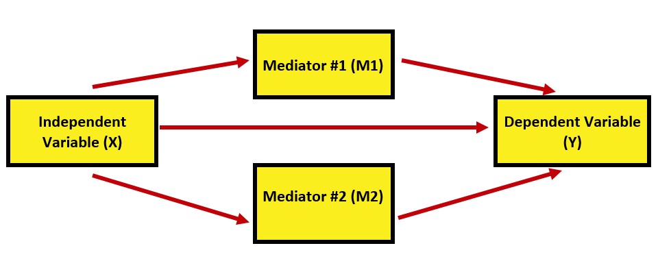
Parallel multiple mediation: An antecedent variable X is modeled as influencing consequent Y directly as well as indirectly through two or more mediators, with the condition that no mediator causally influences another (Hayes, 2022b, p. 161)
With multiple mediation we introduce additional effects:
- Direct effect, \(c'\) (this is not new) quantifies how much two cases that differ by a unit on X are estimated to differ on Y – independent of all mediators.
- Specific indirect effect, \(a_{i}b_{i}\), the individual mediated effects
- Total indirect effects , \(\sum_{i=1}^{k}a_{i}b_{i}\) the sum of the values of the specific indirect effects. The total indirect effect can also be calculated by subtracting the direct effects from the total effects: \(c - c'\)
- Total effect of X on Y, \(c = c' + \sum_{i=1}^{k}a_{i}b_{i}\) (also not new) the sum of the direct and indirect effects. The total effect can also be estimated by regressing Y on X alone.
- Contrasts allow us to directly compare separate mediating effects to see if one indirect effect is stronger than the other.
 In this parallel model, we can describe these effects this way:
- Direct effect: The effect of IV on the DV, accounting for two mediators (indirect effects) in the model.
- Specific indirect effects: There are indirect (or mediating) paths from the IV to the DV; through M1 and M2, respectively.
- Total indirect effect of X on Y: A sum of the value of indirect effects through the specific indirect effects (M1 and M2).
- Total effect: The sum of the direct and indirect effects. Also calculated by regressing Y (dependent variable) on X (independent variable) alone, without any other variables in the model.
Recall that for a complex mediation to be parallel, there can be no causal links between mediators. This is true in this example.
6.4.1 A Mechanical Example
Let’s work a mechanical example with simulated data that assures a statistically significant outcome. Credit to this example is from the Paulo Toffanin website (Toffanin, 2017).
We can bake our own data by updating the script we used in simple mediation to add a second mediator.
6.4.1.1 Data Simulation
# Concerned that identical variable names across book chapters may be
# problematic, I'm adding 'p' in front the 'Data' variable.
set.seed(230925)
X <- rnorm(100)
M1 <- 0.5 * X + rnorm(100)
M2 <- -0.35 * X + rnorm(100)
Y <- 0.7 * M2 + 0.48 * M1 + rnorm(100)
pData <- data.frame(X = X, Y = Y, M1 = M1, M2 = M2)
Using what we learned in conducting a simple mediation in lavaan, we can look at the figure of our proposed model and backwardstrace the paths to write the code.
Remember…
The model exists between 2 single quotation marks (the odd looking ’ and ’ at the beginning and end).
You can write the Y as I have done in the R chunk below, or you can write the Y separately from each arrow, such as
- Y ~ b1*M1
- Y ~ b2*M2
- Y ~ c_p*X
Everything else transfers from our simple mediation, remember that
- the asterisk (“*“) allows us to assign labels (a1, a2, b1, b2, etc.) to the paths; these are helpful for intuitive interpretation
- that eyes/nose notation (:=) is used when creating a new variable that is a function of variables in the model, but not in the dataset (i.e., the a and b path).
- in traditional mediation speak, the direct path from X to Y is c’ (c prime) and the total effect of X to Y (with nothing else in the model) is just c. Hence the c_p label for c prime.
Something new: the contrast statement (only one in this example, but you could have more) allows us to compare the indirect effects to each other. We specify it in the lavaan model, but then need to test it in a subsequent set of script.
Note: In the online example, the writer adds code to correlate M1 and M2. This didn’t/doesn’t seem right to me and then, later, when we amend it to be a serial model, it made even less sense to have them be correlated.
6.4.1.2 Specifying lavaan code
parallel_med <- "
    Y ~ b1*M1 + b2*M2 + c_p*X
    M1 ~ a1*X
    M2 ~ a2*X

    indirect1 := a1 * b1
    indirect2 := a2 * b2
    contrast := indirect1 - indirect2
    total_indirects := indirect1 + indirect2
    total_c    := c_p + (indirect1) + (indirect2)
    direct := c_p
 "
set.seed(230925)  #needed for reproducibility especially when specifying bootstrapped confidence intervals
parallel_fit <- lavaan::sem(parallel_med, data = pData, se = "bootstrap",
    missing = "fiml", bootstrap = 1000)
pfit_sum <- lavaan::summary(parallel_fit, standardized = TRUE, rsq = T,
    fit = TRUE, ci = TRUE)
pfit_ParEsts <- lavaan::parameterEstimates(parallel_fit, boot.ci.type = "bca.simple",
    standardized = TRUE)
pfit_sum
## lavaan 0.6.17 ended normally after 1 iteration
##
## Estimator ML
## Optimization method NLMINB
## Number of model parameters 11
##
## Number of observations 100
## Number of missing patterns 1
##
## Model Test User Model:
##
## Test statistic 2.475
## Degrees of freedom 1
## P-value (Chi-square) 0.116
##
## Model Test Baseline Model:
##
## Test statistic 126.642
## Degrees of freedom 6
## P-value 0.000
##
## User Model versus Baseline Model:
##
## Comparative Fit Index (CFI) 0.988
## Tucker-Lewis Index (TLI) 0.927
##
## Robust Comparative Fit Index (CFI) 0.988
## Robust Tucker-Lewis Index (TLI) 0.927
##
## Loglikelihood and Information Criteria:
##
## Loglikelihood user model (H0) -433.660
## Loglikelihood unrestricted model (H1) -432.423
##
## Akaike (AIC) 889.321
## Bayesian (BIC) 917.977
## Sample-size adjusted Bayesian (SABIC) 883.237
##
## Root Mean Square Error of Approximation:
##
## RMSEA 0.121
## 90 Percent confidence interval - lower 0.000
## 90 Percent confidence interval - upper 0.322
## P-value H_0: RMSEA <= 0.050 0.161
## P-value H_0: RMSEA >= 0.080 0.772
##
## Robust RMSEA 0.121
## 90 Percent confidence interval - lower 0.000
## 90 Percent confidence interval - upper 0.322
## P-value H_0: Robust RMSEA <= 0.050 0.161
## P-value H_0: Robust RMSEA >= 0.080 0.772
##
## Standardized Root Mean Square Residual:
##
## SRMR 0.046
##
## Parameter Estimates:
##
## Standard errors Bootstrap
## Number of requested bootstrap draws 1000
## Number of successful bootstrap draws 1000
##
## Regressions:
## Estimate Std.Err z-value P(>|z|) ci.lower ci.upper
## Y ~
## M1 (b1) 0.456 0.107 4.243 0.000 0.241 0.667
## M2 (b2) 0.743 0.075 9.972 0.000 0.605 0.894
## X (c_p) 0.030 0.099 0.305 0.760 -0.161 0.221
## M1 ~
## X (a1) 0.510 0.081 6.308 0.000 0.353 0.657
## M2 ~
## X (a2) -0.381 0.126 -3.014 0.003 -0.630 -0.129
## Std.lv Std.all
##
## 0.456 0.383
## 0.743 0.693
## 0.030 0.025
##
## 0.510 0.502
##
## -0.381 -0.338
##
## Intercepts:
## Estimate Std.Err z-value P(>|z|) ci.lower ci.upper
## .Y 0.113 0.098 1.155 0.248 -0.088 0.297
## .M1 -0.089 0.099 -0.897 0.370 -0.279 0.098
## .M2 0.017 0.121 0.139 0.889 -0.215 0.273
## Std.lv Std.all
## 0.113 0.083
## -0.089 -0.078
## 0.017 0.013
##
## Variances:
## Estimate Std.Err z-value P(>|z|) ci.lower ci.upper
## .Y 0.855 0.106 8.031 0.000 0.622 1.035
## .M1 0.970 0.118 8.193 0.000 0.728 1.191
## .M2 1.415 0.181 7.815 0.000 1.048 1.742
## Std.lv Std.all
## 0.855 0.465
## 0.970 0.748
## 1.415 0.886
##
## R-Square:
## Estimate
## Y 0.535
## M1 0.252
## M2 0.114
##
## Defined Parameters:
## Estimate Std.Err z-value P(>|z|) ci.lower ci.upper
## indirect1 0.233 0.068 3.435 0.001 0.110 0.376
## indirect2 -0.283 0.094 -3.026 0.002 -0.473 -0.094
## contrast 0.516 0.103 5.001 0.000 0.307 0.712
## total_indircts -0.051 0.127 -0.400 0.689 -0.302 0.198
## total_c -0.021 0.131 -0.157 0.876 -0.277 0.238
## direct 0.030 0.099 0.305 0.760 -0.161 0.221
## Std.lv Std.all
## 0.233 0.192
## -0.283 -0.234
## 0.516 0.426
## -0.051 -0.042
## -0.021 -0.017
## 0.030 0.025## lhs op rhs label est se
## 1 Y ~ M1 b1 0.456 0.107
## 2 Y ~ M2 b2 0.743 0.075
## 3 Y ~ X c_p 0.030 0.099
## 4 M1 ~ X a1 0.510 0.081
## 5 M2 ~ X a2 -0.381 0.126
## 6 Y ~~ Y 0.855 0.106
## 7 M1 ~~ M1 0.970 0.118
## 8 M2 ~~ M2 1.415 0.181
## 9 X ~~ X 1.253 0.000
## 10 Y ~1 0.113 0.098
## 11 M1 ~1 -0.089 0.099
## 12 M2 ~1 0.017 0.121
## 13 X ~1 0.009 0.000
## 14 indirect1 := a1*b1 indirect1 0.233 0.068
## 15 indirect2 := a2*b2 indirect2 -0.283 0.094
## 16 contrast := indirect1-indirect2 contrast 0.516 0.103
## 17 total_indirects := indirect1+indirect2 total_indirects -0.051 0.127
## 18 total_c := c_p+(indirect1)+(indirect2) total_c -0.021 0.131
## 19 direct := c_p direct 0.030 0.099
## z pvalue ci.lower ci.upper std.lv std.all std.nox
## 1 4.243 0.000 0.227 0.658 0.456 0.383 0.383
## 2 9.972 0.000 0.597 0.890 0.743 0.693 0.693
## 3 0.305 0.760 -0.160 0.227 0.030 0.025 0.022
## 4 6.308 0.000 0.356 0.660 0.510 0.502 0.448
## 5 -3.014 0.003 -0.624 -0.125 -0.381 -0.338 -0.302
## 6 8.031 0.000 0.671 1.078 0.855 0.465 0.465
## 7 8.193 0.000 0.758 1.248 0.970 0.748 0.748
## 8 7.815 0.000 1.113 1.834 1.415 0.886 0.886
## 9 NA NA 1.253 1.253 1.253 1.000 1.253
## 10 1.155 0.248 -0.078 0.301 0.113 0.083 0.083
## 11 -0.897 0.370 -0.286 0.094 -0.089 -0.078 -0.078
## 12 0.139 0.889 -0.234 0.240 0.017 0.013 0.013
## 13 NA NA 0.009 0.009 0.009 0.008 0.009
## 14 3.435 0.001 0.124 0.395 0.233 0.192 0.172
## 15 -3.026 0.002 -0.483 -0.105 -0.283 -0.234 -0.209
## 16 5.001 0.000 0.299 0.708 0.516 0.426 0.380
## 17 -0.400 0.689 -0.304 0.193 -0.051 -0.042 -0.037
## 18 -0.157 0.876 -0.251 0.252 -0.021 -0.017 -0.015
## 19 0.305 0.760 -0.160 0.227 0.030 0.025 0.0226.4.1.3 A note on indirect effects and confidence intervals
Before we move onto interpretation, I want to stop and look at both \(p\) values and confidence intervals. Especially with Hayes (2022b) PROCESS macro, there is a great deal of emphasis on the use of bootstrapped confidence intervals to determine the statistical significance of the indirect effects. In fact, PROCESS output has (at least historically) not provided \(p\) values with the indirect effects. This is because, especially in the ordinary least squares context, bias-corrected bootstrapped confidence intervals are more powerful (i.e., they are more likely to support a statistically significant result) than \(p\) values.
An excellent demonstration of this phenomena was provided by Mallinckrodt et al. (2006) where they compared confidence intervals produced by the normal theory method to those that are bias corrected. The bias corrected intervals were more powerful to determining if there were statistically significant indirect effects.
The method we have specified in lavaan produced bias-corrected confidence intervals. The \(p\) values and corresponding confidence intervals should be consistent with each other. That is, if \(p\) < .05, then the CI95s should not pass through zero. Of course we can always check to be certain this is true. For this reason, I will report \(p\) values in my results. There are reviewers, though, who may prefer that you report CI95s (or both).
6.4.1.4 Figures and Tables
To assist in table preparation, it is possible to export the results to a .csv file that can be manipulated in Excel, Microsoft Word, or other program to prepare an APA style table.
We can use the package tidySEM to create a figure that includes the values on the path.
Here’s what the base package gets us
# only worked when I used the library to turn on all these pkgs
library(lavaan)
library(dplyr)
library(ggplot2)
library(tidySEM)
tidySEM::graph_sem(model = parallel_fit)
We can create model that communicates more intuitively with a little tinkering. First, let’s retrieve the current “map” of the layout.
##      [,1] [,2] [,3]
## [1,] NA   "X"  NA
## [2,] "M1" "M2" "Y"
## attr(,"class")
## [1] "layout_matrix" "matrix"        "array"
To create the figure I showed at the beginning of the chapter, we will want three rows and three columns.
parallel_map <- tidySEM::get_layout("", "M1", "", "X", "", "Y", "", "M2",
    "", rows = 3)
parallel_map
## [,1] [,2] [,3]
## [1,] "" "M1" ""
## [2,] "X" "" "Y"
## [3,] "" "M2" ""
## attr(,"class")
## [1] "layout_matrix" "matrix" "array"We can update our figure by supplying this new map and adjusting the object and text sizes.
tidySEM::graph_sem(parallel_fit, layout = parallel_map, rect_width = 1.5,
    rect_height = 1.25, spacing_x = 2, spacing_y = 3, text_size = 4.5)
There are a number of ways to tabalize the data. You might be surprised to learn that a number of articles that analyze mediating effects focus their presentation on those values and not the traditional intercepts and B weights. This is the approach I have taken in this chapter.
Table 1
| Model Coefficients Assessing M1 and M2 as Parallel Mediators Between X and Y |
|---|
| Predictor | \(B\) | \(SE_{B}\) | \(p\) | \(R^2\) |
|---|
| M1 | .25 | |||
|---|---|---|---|---|
| Constant | -0.089 | 0.099 | 0.370 | |
| X (\(a_1\)) | 0.510 | 0.081 | <0.001 |
| M2 | .11 | |||
|---|---|---|---|---|
| Constant | 0.017 | 0.121 | 0.889 | |
| X (\(a_2\)) | -0.381 | 0.126 | 0.003 |
| DV | .54 | |||
|---|---|---|---|---|
| Constant | 0.113 | 0.098 | 0.248 | |
| M1 (\(b_1\)) | 0.456 | 0.107 | <0.001 | |
| M2 (\(b_2\)) | 0.743 | 0.075 | <0.001 | |
| X (\(c'\)) | 0.030 | 0.099 | 0.760 |
| Summary of Effects | \(B\) | \(SE_{B}\) | \(p\) | 95% CI |
|---|---|---|---|---|
| Total | -0.021 | 0.131 | 0.876 | -0.251, 0.252 |
| Indirect 1 (\(a_1\) * \(a_2\)) | 0.233 | 0.068 | 0.001 | 0.124, 0.395 |
| Indirect 2 (\(b_1\) * \(b_2\)) | -0.283 | 0.094 | 0.002 | -0.483, -0.105 |
| Total indirects | -0.051 | 0.127 | 0.689 | -0.304, 0.193 |
| Contrast (Ind1 - Ind2) | 0.516 | 0.103 | <0.001 | 0.299, 0.708 |
| Note. The significance of the indirect effects was calculated with bootstrapped, bias-corrected, confidence intervals (.95). |
6.4.1.5 APA Style Writeup
You may notice that my write-up includes almost no statistical output. This is consistent with APA style that avoids redundancy in text and table. When I want to emphasize a specific result, I may duplicate some output in the text.
A model of parallel multiple mediation was analyzed examining the degree to which importance of M1 and M2 mediated the relation of X on Y. Hayes (2022b) recommended this strategy over simple mediation models because it allows for all mediators to be examined, simultaneously. The resultant direct and indirect values for each path account for other mediation paths. Using the lavaan (v. 0.6-16) package in R, coefficients for specific indirect, total indirect, direct, and total were computed. Path coefficients refer to regression weights, or slopes, of the expected changes in the dependent variable given a unit change in the independent variables.
Results (depicted in Figure 1 and presented in Table 1) suggest that 54% of the variance in Y is accounted for by the model. Neither the total nor direct effect of X on Y were statistically significant. In contrast, both indirect effects were statistically significant. A pairwise comparison of the specific indirect effects indicated that the strength of the effects were statistically significantly different from each other. In summary, the effect of X on Y is mediated through M1 and M2, with a stronger influence through M2.
You may notice this write-up included only one statistic. I offered this as an example of avoiding redundancy in text and table. When tables and figures convey maximal information, the results section may be used to describe the patterns – including numbers when they reduce the cognitive load for the readers and reviewers.
Let’s turn now to the research vignette and work an example with simulated data from that example. Because the research vignette use an entirely new set of output I will either restart R or clear my environment so that there are a few less objects “in the way.”
6.4.2 Research Vignette
The research vignette comes from the Lewis, Williams, Peppers, and Gadson’s (2017) study titled, “Applying Intersectionality to Explore the Relations Between Gendered Racism and Health Among Black Women.” The study was published in the Journal of Counseling Psychology. Participants were 231 Black women who completed an online survey.
Variables used in the study included:
GRMS: Gendered Racial Microaggressions Scale (J. A. Lewis & Neville, 2015) is a 26-item scale that assesses the frequency of nonverbal, verbal, and behavioral negative racial and gender slights experienced by Black women. Scaling is along six points ranging from 0 (never) to 5 (once a week or more). Higher scores indicate a greater frequency of gendered racial microaggressions. An example item is, “Someone has tried to ‘put me in my place.’”
MntlHlth and PhysHlth: Short Form Health Survey - Version 2 (Ware et al., 1995) is a 12-item scale used to report self-reported mental (six items) and physical health (six items). Although the article did not specify, when this scale is used in other contexts (e.g., Paul Youngbin Kim et al., 2017), a 6-point scale has been reported. Higher scores indicate higher mental health (e.g., little or no psychological distress) and physical health (e.g., little or no reported symptoms in physical functioning). An example of an item assessing mental health was, “How much of the time during the last 4 weeks have you felt calm and peaceful?”; an example of a physical health item was, “During the past 4 weeks, how much did pain interfere with your normal work?”
Sprtlty, SocSup, Engmgt, and DisEngmt are four subscales from the Brief Coping with Problems Experienced Inventory (Carver, 1997). The 28 items on this scale are presented on a 4-point scale ranging from 1 (I usually do not do this at all) to 4(I usually do this a lot). Higher scores indicate a respondents’ tendency to engage in a particular strategy. Instructions were modified to ask how the female participants responded to recent experiences of racism and sexism as Black women. The four subscales included spirituality (religion, acceptance, planning), interconnectedness/social support (vent emotions, emotional support,instrumental social support), problem-oriented/engagement coping (active coping, humor, positive reinterpretation/positive reframing), and disengagement coping (behavioral disengagement, substance abuse, denial, self-blame, self-distraction).
GRIcntlty: The Multidimensional Inventory of Black Identity Centrality subscale (Sellers et al., n.d.) was modified to measure the intersection of racial and gender identity centrality. The scale included 10 items scaled from 1 (strongly disagree) to 7 (strongly agree). An example item was, “Being a Black woman is important to my self-image.” Higher scores indicated higher levels of gendered racial identity centrality.
6.4.2.1 Data Simulation
The lavaan::simulateData function was used. If you have taken psychometrics, you may recognize the code as one that creates latent variables form item-level data. In trying to be as authentic as possible, we retrieved factor loadings from psychometrically oriented articles that evaluated the measures (Nadal, 2011; Veit & Ware, 1983). For all others we specified a factor loading of 0.80. We then approximated the measurement model by specifying the correlations between the latent variable. We sourced these from the correlation matrix from the research vignette (J. A. Lewis et al., 2017). The process created data with multiple decimals and values that exceeded the boundaries of the variables. For example, in all scales there were negative values. Therefore, the final element of the simulation was a linear transformation that rescaled the variables back to the range described in the journal article and rounding the values to integer (i.e., with no decimal places).
#Entering the intercorrelations, means, and standard deviations from the journal article

Lewis_generating_model <- '
        ##measurement model
        GRMS  =~ .69*Ob1 + .69*Ob2 + .60*Ob3 + .59*Ob4 + .55*Ob5 + .55*Ob6 + .54*Ob7 + .50*Ob8 + .41*Ob9 + .41*Ob10 + .93*Ma1 + .81*Ma2 + .69*Ma3 + .67*Ma4 + .61*Ma5 + .58*Ma6 + .54*Ma7 + .59*St1 + .55*St2 + .54*St3 + .54*St4 + .51*St5 + .70*An1 + .69*An2 + .68*An3
        MntlHlth  =~ .8*MH1 + .8*MH2 + .8*MH3 + .8*MH4 + .8*MH5 + .8*MH6
        PhysHlth  =~ .8*PhH1 + .8*PhH2 + .8*PhH3 + .8*PhH4 + .8*PhH5 + .8*PhH6
        Spirituality  =~ .8*Spirit1 + .8*Spirit2
        SocSupport  =~ .8*SocS1 + .8*SocS2
        Engagement  =~ .8*Eng1 + .8*Eng2
        Disengagement  =~  .8*dEng1 + .8*dEng2
        GRIC  =~ .8*Cntrlty1 + .8*Cntrlty2 + .8*Cntrlty3 + .8*Cntrlty4 + .8*Cntrlty5 + .8*Cntrlty6 + .8*Cntrlty7 + .8*Cntrlty8 + .8*Cntrlty9 + .8*Cntrlty10

        # Means
         GRMS ~ 1.99*1
         Spirituality ~2.82*1
         SocSupport ~ 2.48*1
         Engagement ~ 2.32*1
         Disengagement ~ 1.75*1
         GRIC ~ 5.71*1
         MntlHlth ~3.56*1 #Lewis et al used sums instead of means, I recast as means to facilitate simulation
         PhysHlth ~ 3.51*1 #Lewis et al used sums instead of means, I recast as means to facilitate simulation

        # Correlations
         GRMS ~ 0.20*Spirituality
         GRMS ~ 0.28*SocSupport
         GRMS ~ 0.30*Engagement
         GRMS ~ 0.41*Disengagement
         GRMS ~ 0.19*GRIC
         GRMS ~ -0.32*MntlHlth
         GRMS ~ -0.18*PhysHlth

         Spirituality ~ 0.49*SocSupport
         Spirituality ~ 0.57*Engagement
         Spirituality ~ 0.22*Disengagement
         Spirituality ~ 0.12*GRIC
         Spirituality ~ -0.06*MntlHlth
         Spirituality ~ -0.13*PhysHlth

         SocSupport ~ 0.46*Engagement
         SocSupport ~ 0.26*Disengagement
         SocSupport ~ 0.38*GRIC
         SocSupport ~ -0.18*MntlHlth
         SocSupport ~ -0.08*PhysHlth

         Engagement ~ 0.37*Disengagement
         Engagement ~ 0.08*GRIC
         Engagement ~ -0.14*MntlHlth
         Engagement ~ -0.06*PhysHlth

         Disengagement ~ 0.05*GRIC
         Disengagement ~ -0.54*MntlHlth
         Disengagement ~ -0.28*PhysHlth

         GRIC ~ -0.10*MntlHlth
         GRIC ~ 0.14*PhysHlth

         MntlHlth ~ 0.47*PhysHlth
        '

set.seed(230925)
dfLewis <- lavaan::simulateData(model = Lewis_generating_model,
                              model.type = "sem",
                              meanstructure = T,
                              sample.nobs=231,
                              standardized=FALSE)

#used to retrieve column indices used in the rescaling script below
#col_index <- as.data.frame(colnames(dfLewis))

for(i in 1:ncol(dfLewis)){  # for loop to go through each column of the dataframe
  if(i >= 1 & i <= 25){   # apply only to GRMS variables
    dfLewis[,i] <- scales::rescale(dfLewis[,i], c(0, 5))
  }
  if(i >= 26 & i <= 37){   # apply only to mental and physical health variables
    dfLewis[,i] <- scales::rescale(dfLewis[,i], c(0, 6))
  }
  if(i >= 38 & i <= 45){   # apply only to coping variables
    dfLewis[,i] <- scales::rescale(dfLewis[,i], c(1, 4))
  }
  if(i >= 46 & i <= 55){   # apply only to GRIC variables
    dfLewis[,i] <- scales::rescale(dfLewis[,i], c(1, 7))
  }
}

#rounding to integers so that the data resembles that which was collected
library(tidyverse)
dfLewis <- dfLewis %>% round(0)

#quick check of my work
#psych::describe(dfLewis)
The script below allows you to store the simulated data as a file on your computer. This is optional – the entire lesson can be worked with the simulated data.
If you prefer the .rds format, use this script (remove the hashtags). The .rds format has the advantage of preserving any formatting of variables. A disadvantage is that you cannot open these files outside of the R environment.
Script to save the data to your computer as an .rds file.
Once saved, you could clean your environment and bring the data back in from its .csv format.
If you prefer the .csv format (think “Excel lite”) use this script (remove the hashtags). An advantage of the .csv format is that you can open the data outside of the R environment. A disadvantage is that it may not retain any formatting of variables
Script to save the data to your computer as a .csv file.
Once saved, you could clean your environment and bring the data back in from its .csv format.
6.4.3 Scrubbing, Scoring, and Data Diagnostics
Because the focus of this lesson is on complex mediation, we have used simulated data. If this were real, raw, data, it would be important to scrub, score, and conduct data diagnostics to evaluate the suitability of the data for the proposes anlayses.
Because we are working with item level data we do need to score the scales used in the researcher’s model. Because we are using simulated data and the authors already reverse coded any such items, we will omit that step.
As described in the Scoring chapter, we calculate mean scores of these variables by first creating concatenated lists of variable names. Next we apply the sjstats::mean_n function to obtain mean scores when a given percentage (we’ll specify 80%) of variables are non-missing. Functionally, this would require the two-item variables (e.g., engagement coping and disengagement coping) to have non-missingness. We simulated a set of data that does not have missingness, none-the-less, this specification is useful in real-world settings.
Note that I am only scoring the variables used in the models demonstrated in this lesson. The remaining variables are available as practice options.
GRMS_vars <- c("Ob1", "Ob2", "Ob3", "Ob4", "Ob5", "Ob6", "Ob7", "Ob8",
    "Ob9", "Ob10", "Ma1", "Ma2", "Ma3", "Ma4", "Ma5", "Ma6", "Ma7", "St1",
    "St2", "St3", "St4", "St5", "An1", "An2", "An3")
Eng_vars <- c("Eng1", "Eng2")
dEng_vars <- c("dEng1", "dEng2")
MntlHlth_vars <- c("MH1", "MH2", "MH3", "MH4", "MH5", "MH6")

dfLewis$GRMS <- sjstats::mean_n(dfLewis[, GRMS_vars], 0.8)
dfLewis$Engmt <- sjstats::mean_n(dfLewis[, Eng_vars], 0.8)
dfLewis$DisEngmt <- sjstats::mean_n(dfLewis[, dEng_vars], 0.8)
dfLewis$MntlHlth <- sjstats::mean_n(dfLewis[, MntlHlth_vars], 0.8)

# If the scoring code above does not work for you, try the format
# below which involves inserting to periods in front of the variable
# list. One example is provided. dfLewis$GRMS <-
# sjstats::mean_n(dfLewis[, ..GRMS_vars], 0.80)
Now that we have scored our data, let’s trim the variables to just those we need.
Let’s check a table of means, standard deviations, and correlations to see if they align with the published article.
Lewis_table <- apaTables::apa.cor.table(Lewis_df, table.number = 1, show.sig.stars = TRUE,
    landscape = TRUE, filename = "Lewis_Corr.doc")
print(Lewis_table)
##
##
## Table 1
##
## Means, standard deviations, and correlations with confidence intervals
##
##
## Variable M SD 1 2 3
## 1. GRMS 2.56 0.72
##
## 2. Engmt 2.48 0.53 .52**
## [.42, .61]
##
## 3. DisEngmt 2.48 0.52 .53** .32**
## [.43, .62] [.20, .43]
##
## 4. MntlHlth 3.16 0.81 -.56** -.23** -.48**
## [-.64, -.47] [-.35, -.11] [-.57, -.37]
##
##
## Note. M and SD are used to represent mean and standard deviation, respectively.
## Values in square brackets indicate the 95% confidence interval.
## The confidence interval is a plausible range of population correlations
## that could have caused the sample correlation (Cumming, 2014).
## * indicates p < .05. ** indicates p < .01.
## While they are not exact, they approximate the magnitude and patterns in the correlation matrix in the article (J. A. Lewis et al., 2017).
6.4.3.1 Specifying the lavaan model
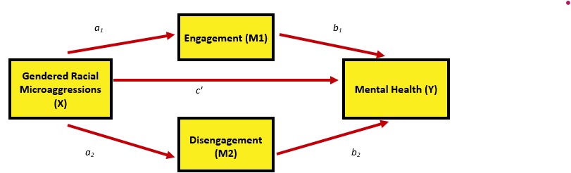
The Lewis et al. article (2017) reports four mediation analyses, each repeated for mental and physical outcomes. Thus, their write-up reports eight simple mediation models. Graphically, their analyses were efficiently presented in a figure that looked (to me) like parallel mediation. Correspondingly, it made sense to me that we could try this in our research vignette. In the upcoming chapter on conditional process analysis, we will work the moderated mediation that was a primary focus of their research.
Below is the model we will work. Specifically, we will evaluate whether gendered racial microaggressions impact mental health separately, thorough mediated paths of engagement and disengagement. We will also be able to see if the strength of those mediated paths are statistically, significantly, different from each other.
We can use the guidelines above to specify our model and then request summaries of the fit indices and parameter estimates.
parallel_Lewis <- "
    MntlHlth ~ b1*Engmt + b2*DisEngmt + c_p*GRMS
    Engmt ~ a1*GRMS
    DisEngmt ~ a2*GRMS

    indirect1 := a1 * b1
    indirect2 := a2 * b2
    contrast := indirect1 - indirect2
    total_indirects := indirect1 + indirect2
    total_c := c_p + (indirect1) + (indirect2)
    direct := c_p
"
set.seed(230925)  #necessary for reproducible results because lavaan introduces randomness into the estimation process
para_Lewis_fit <- lavaan::sem(parallel_Lewis, data = Lewis_df, se = "bootstrap",
    bootstrap = 1000, missing = "fiml")  #holds the 'whole' result
pLewis_sum <- lavaan::summary(para_Lewis_fit, standardized = TRUE, rsq = T,
    fit = TRUE, ci = TRUE)  #today, we really only need the R-squared from here
pLewis_ParEsts <- lavaan::parameterEstimates(para_Lewis_fit, boot.ci.type = "bca.simple",
    standardized = TRUE)  #provides our estimates, se, p values for all the elements we specified

pLewis_sum
pLewis_ParEsts
6.4.3.2 Table and Figure
To assist in table preparation, it is possible to export the results to a .csv file that can be manipulated in Excel, Microsoft Word, or other program to prepare an APA style table.
We can use the package tidySEM to create a figure that includes the values on the path.
Here’s what the base package gets us
# only worked when I used the library to turn on all these pkgs
library(lavaan)
library(dplyr)
library(ggplot2)
library(tidySEM)
tidySEM::graph_sem(model = para_Lewis_fit)
We can create model that communicates more intuitively with a little tinkering. First, let’s retrieve the current “map” of the layout.
##      [,1]    [,2]       [,3]
## [1,] NA      "GRMS"     NA
## [2,] "Engmt" "DisEngmt" "MntlHlth"
## attr(,"class")
## [1] "layout_matrix" "matrix"        "array"
To create the figure I showed at the beginning of the chapter, we will want three rows and three columns.
pLewis_map <- tidySEM::get_layout("", "Engmt", "", "GRMS", "", "MntlHlth",
    "", "DisEngmt", "", rows = 3)
pLewis_map
## [,1] [,2] [,3]
## [1,] "" "Engmt" ""
## [2,] "GRMS" "" "MntlHlth"
## [3,] "" "DisEngmt" ""
## attr(,"class")
## [1] "layout_matrix" "matrix" "array"We can update our figure by supplying this new map and adjusting the object and text sizes.
tidySEM::graph_sem(para_Lewis_fit, layout = pLewis_map, rect_width = 1.5,
    rect_height = 1.25, spacing_x = 2, spacing_y = 3, text_size = 4.5)
Now let’s make a table.
Table 2
| Model Coefficients Assessing Engagement and Disengagement Coping as Parallel Mediators Between Predicting Mental Health from Gendered Racial Microaggressions |
|---|
| Predictor | \(B\) | \(SE_{B}\) | \(p\) | \(R^2\) |
|---|
| Engagement coping (M1) | .27 | |||
|---|---|---|---|---|
| Constant | 1.494 | 0.111 | <0.001 | |
| GRMS (\(a_1\)) | 0.384 | 0.042 | <0.001 |
| Disengagement coping (M2) | .28 | |||
|---|---|---|---|---|
| Constant | 1.490 | 0.100 | <0.001 | |
| GRMS (\(a_2\)) | 0.386 | 0.038 | <0.001 |
| Mental Health (DV) | .37 | |||
|---|---|---|---|---|
| Constant | 5.141 | 0.226 | <0.001 | |
| Engagement (\(b_1\)) | 0.144 | 0.089 | 0.106 | |
| Disengagement (\(b_2\)) | -0.391 | 0.089 | <0.001 | |
| GRMS (\(c'\)) | -0.535 | 0.076 | <0.001 |
| Summary of Effects | \(B\) | \(SE_{B}\) | \(p\) | 95% CI |
|---|---|---|---|---|
| Total | -0.631 | 0.058 | <0.001 | -0.739, -0.505 |
| Indirect 1 (\(a_1\) * \(a_2\)) | 0.055 | 0.036 | 0.121 | -0.003, 0.140 |
| Indirect 2 (\(b_1\) * \(b_2\)) | -0.151 | 0.038 | <0.001 | -0.235, -0.085 |
| Total indirects | -0.096 | 0.051 | 0.059 | -0.193, 0.007 |
| Contrast (Ind1 - Ind2) | 0.206 | 0.054 | <0.001 | 0.109, 0.338 |
| Note. GRMS = gendered racial microaggressions. The significance of the indirect effects was calculated with bootstrapped, bias-corrected, confidence intervals (.95). |
- The model accounts for 37% of the variance in predicting mental health outcomes.
- The total effect of GRMS on mental health is -0.631 (\(p < 0.001\)) is negative and statistically significant. That is, gendered racial microaggressions have a statistically significant negative effect on mental health.
- The direct effect of GRMS on mental health is -0.535 (\(p < 0.001\)); while this is lower than the total effect, it remains statistically significant.
- Using Baron and Kenny’s (1986) causal steps logic, the fact that the direct effect does not decrease in a statistically significant manner does not provide helpful, logical support for mediation. According to Hayes (2022b) this difference is not necessary. That is, a statistically significant indirect effect can stand on its own.
- Indirect effect #1 (a1 x b1 or GRMS through engagement coping) is 0.055 (\(p = 0.121, CI95[-0.003, 0.140]\)) and not statistically significant. Because they can be inconsistent with the p values, we should always check the confidence intervals to see if they pass through zero. In this case they do.
- Indirect effect #2 (a2 x b2, or GRMS through disengagement to coping) is -0.151 (\(p < 0.001, CI95[-0.235, -0.085]\)). The p value is significant and the 95% confidence interval does not pass through zero. Thus, gendered racial microaggressions lead to greater disengagement (a1). In turn, disengagement has negative effects on mental health (b2).
- The total indirect effect (i.e., sum of all specific indirect effects) \((-0.096, p = 0.059)\) is not statistically significant.
- We examine the contrast to see if the indirect effects statistically significantly different from each other: \(B= 0.206, p < 0.001\). They are. This is not surprising since the path mediated by engagement was not statistically significant but the path mediated by disengagement was statistically significant.
6.4.3.3 APA Style Writeup
Hayes (Hayes, 2022a) provides helpful guidelines for presenting statistical results. Here is a summary of his recommendations.
- Pack as much statistical info as possible into a table(s) or figure(s).
- Use statistics in the text as punctuation; avoid redundancy in text and table.
- Avoid using abbreviations for variables in the text itself; rather focus on the construct names rather than their shorthand
- Avoid focusing on what you hypothesized (e.g., avoid, “Results supported/did not support hypothesis A1”) and instead focus on what you found. The reader is more interested in the results, not your forecasts.
- Hayes prefers reporting unstandardized metrics because they map onto the measurement scales used in the study. He believes this is especially important when dichotomous variables are used.
- There is “no harm” in reporting hypothesis tests and CIs for the a and b paths, but whether/not these paths are statistically significant does not determine the significance of the indirect effect.
- Be precise with language:
- OK: X exerts an effect on Y directly and/or indirectly through M.
- Not OK: the indirect effect of M
- Report direct and indirect effects and their corresponding inferential tests
- Hayes argues that a statistically significant indirect effect is, in fact statistic. He dislikes narration of the Baron and Kenny (1986) process and steps.
Here’s my attempt to write up the simulated data from the Lewis et al. (2017) article.
Method
Data Analysis
Parallel multiple mediation is appropriate when testing the influence of an independent variable (X) on the dependent variable (Y) directly, as well as indirectly through two or more mediators. A condition of parallel multiple mediation is that no mediator causally influences another (Hayes, 2022b). Using data simulated from Lewis et al. (2017) we utilized parallel multiple mediation analysis to test the influence of gendered racial microaggressions (X, GRMS) on mental health outcomes (Y, MntlHlth) directly as well as indirectly through the mediators engagement coping (M1, Engmt) and disengaged coping (M2, DisEngmt). Using the lavaan (v. 0.6-16) package in R we followed the procedures outlined in Hayes (2022b) by analyzing the strength and significance of four sets of effects: specific indirect, the total indirect, the direct, and total.
Results
Preliminary Analyses Descriptive statistics were computed, and all variables were assessed for skewness and kurtosis. More narration,here. A summary of descriptive statistics and a correlation matrix for the study is provided in Table 2. These bivariate relations provide evidence to support the test of mediation analysis.
Parallel Multiple Mediation Analysis A model of parallel mediation examined the degree to which engagement and disengagement coping strategies mediated the relation of gendered racial microaggressions on mental health outcomes in Black women. Hayes (2022b) recommended this strategy over simple mediation models because it allows for all mediators to be examined, simultaneously. The resultant direct and indirect values for each path account for other mediation paths. Using the lavaan (v. 0.6-17) package in R, coefficients for specific indirect, total indirect, direct, and total were computed. Path coefficients refer to regression weights, or slopes, of the expected changes in the dependent variable given a unit change in the independent variables.
Results (depicted in Figure 2 and presented in Table 3) suggest that 37% of the variance in mental health outcomes is accounted for by the model. The indirect effect predicting mental health from gendered racial microaggressions via engagement coping was not statistically significant \(*B = 0.055, SE = 0.036, p = 0.121, CI95[-0.003, 0.140 ]\)). Looking at the individual paths we see that \(a_{1}\) was positive and statistically significant (GRMS leds to increased engagement coping), but the subsequent link, \(b_{1}\) (engagement to mental health) was not. The indirect effect predicting mental health from gendered racial microaggressions through disengagement to coping was statistically significant \(B = -0.151, SE = 0.038, p < 0.001, CI95[-0.235, -0.085]\)). In this case, gendered racial microaggressions led to greater disengagement coping (\(a_{2}\)). In turn, disengagement coping had negative effects on mental health (\(b_{2}\)). Curiously, the total indirect effect (i.e., the sum of the specific indirect effects was not statistically significant. It is possible that the positive and negative valences of the indirect effects “cancelled each other out.” A pairwise comparison of the specific indirect effects indicated that the strength of the effects were statistically significantly different from each other. Given that the path through engagement coping was not significant, but the path through disengagement coping was, this statistically significant difference is not surprising.
Hints for Writing Method/Results Sections
- When you find an article you like, make note of it and put it in a very special folder. In recent years, I have learned to rely on full-text versions stored in my Zotero app.
- Once you know your method (measure, statistic, etc.) begin collecting others articles that are similar to it. To write results sections I will often reference multiple articles.
- When it iss time to write have all these resources handy and use them as guides/models.
- Put as much info as possible in the table. Become a table-pro. That is, learn how to merge/split cells, use borders/shading, the decimal tab, and so forth. Don’t make the borders disappear until the last thing you do before submitting. This is because you ALWAYS have to update your tables and seeing the borders makes it easier.
6.5 Serial Multiple Mediator Model
Recall that one of the conditions of the parallel mediator model was that “no mediator causally influences another.”
Regarding these correlated mediators (Hayes, 2022b):
- Typically, two or more mediators that are causally located between X and Y will be correlated - if for no other reason than that they share a common cause (X).
- Estimating the partial correlation between two mediators after controlling for X is one way to examine whether all of their association is accounted for by this common cause.
- Partial correlation is the Pearson correlation between the residuals from a model estimating Y from a set of covariates, and the residuals from a model estimating X from the same set of covariates.
- Partial correlations allow the assessment of their association, independent of what they have in common with the covariates that were regressed onto Y and X, separately.
- If two (or more) mediators remain correlated after adjusting for X, then
- the correlation is spurious, they share another (unmodeled) common cause.
- the remaining association is epiphenomenal. That is, a proposed mediator could be related to an outcome not because it causes the outcome, but because it is correlated with another variable that is causally influencing the outcome. This is a noncausal alternative explanation for an association. Also, many things correlated with the cause of Y will also tend to be correlated with X, but it doesn’t make all those things cause Y
- or one mediator causally affects another
The goal of a serial multiple mediator model is to investigate the direct and indirect effects of X on Y while modeling a process in which X causes M1, which in turn causes M2, and so forth, concluding with Y as the final consequent.
As before, we will calculate:
- Direct effect, c’: the estimated difference in Y between two cases that differ by one unit on X but who are equal on all mediators in the model.
- Specific indirect effects, a1b1, a2b2, a3b3, etc.: constructed by multiplying the regression weights corresponding to each step in an indirect pathway; interpreted as the estimated difference in Y between two cases that differ by one unit on X through the causal sequence from X to mediator(s) to Y.
- Total indirect effect of X: sum of all specific indirect effects
- Total effect of X: the total indirect effect of X plus the direct effect of X; can also be estimated by regressing Y from X only.
- Pairwise comparisons (contrasts) between indirect effects (i.e., is one indirect effect stronger than another)
6.5.1 We stick with the Lewis et al. (2017) example, but modify it.
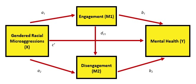
Our parallel multiple mediator model of gendered racial microaggressions on mental health through engagement and disengagement coping strategies assumed no causal association between the mediators. Noting the statistically significant correlation between engagement and disengagement, what if engagement influenced disengagement, which, in turn influenced mental health.
If this is our goal (image), how many direct and indirect effects are contained in this model? Using the same processes as before, let’s plan our model:
- We add a path predicting disengagement from engagement, and label it with a \(d_{21}\)
- Regarding the notation, it makes sense that we use a d to designate a new type of path; I don’t know why we use a subscript of 21
- We specify a third indirect path that multiplies those 3 paths (a1, d21, b2) together
- We add a third contrast so that we get all the combinations of indirect comparisons: 1-2, 1-3 2-3
- We update our total_indirects calculation to include indirect#3
- We update our total_c calculation to include indirect#3
6.5.2 Specify the lavaan model
serial_Lewis <- "
    MntlHlth ~ b1*Engmt + b2*DisEngmt + c_p*GRMS
    Engmt ~ a1*GRMS
    DisEngmt ~ a2*GRMS
    DisEngmt ~ d21*Engmt

    indirect1 := a1 * b1
    indirect2 := a2 * b2
    indirect3 := a1 * d21 * b2
    contrast1 := indirect1 - indirect2
    contrast2 := indirect1 - indirect3
    contrast3 := indirect2 - indirect3
    total_indirects := indirect1 + indirect2 + indirect3
    total_c := c_p + indirect1 + indirect2 + indirect3
    direct := c_p
"
set.seed(230925)  #necessary for reproducible results because lavaan introduces randomness into the estimation process
serial_Lewis_fit <- lavaan::sem(serial_Lewis, data = Lewis_df, se = "bootstrap",
    missing = "fiml", bootstrap = 1000)
sLewis_sum <- lavaan::summary(serial_Lewis_fit, standardized = TRUE, rsq = T,
    fit = TRUE, ci = TRUE)
sLewis_ParEsts <- lavaan::parameterEstimates(serial_Lewis_fit, boot.ci.type = "bca.simple",
    standardized = TRUE)

sLewis_sum
sLewis_ParEsts
6.5.2.1 Table and Figure
To assist in table preparation, it is possible to export the results to a .csv file that can be manipulated in Excel, Microsoft Word, or other program to prepare an APA style table.
We can use the package tidySEM to create a figure that includes the values on the path.
Here’s what the base package gets us
# only worked when I used the library to turn on all these pkgs
library(lavaan)
library(dplyr)
library(ggplot2)
library(tidySEM)
tidySEM::graph_sem(model = serial_Lewis_fit)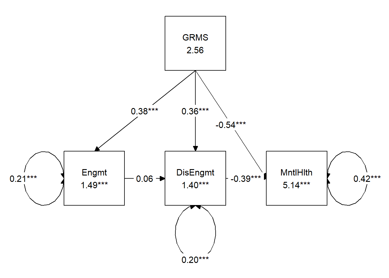
We can create model that communicates more intuitively with a little tinkering. First, let’s retrieve the current “map” of the layout.
##      [,1]    [,2]       [,3]
## [1,] NA      "GRMS"     NA
## [2,] "Engmt" "DisEngmt" "MntlHlth"
## attr(,"class")
## [1] "layout_matrix" "matrix"        "array"
To create the figure I showed at the beginning of the chapter, we will want three rows and three columns.
sLewis_map <- tidySEM::get_layout("", "Engmt", "", "GRMS", "", "MntlHlth",
    "", "DisEngmt", "", rows = 3)
sLewis_map
## [,1] [,2] [,3]
## [1,] "" "Engmt" ""
## [2,] "GRMS" "" "MntlHlth"
## [3,] "" "DisEngmt" ""
## attr(,"class")
## [1] "layout_matrix" "matrix" "array"We can update our figure by supplying this new map and adjusting the object and text sizes.
tidySEM::graph_sem(serial_Lewis_fit, layout = sLewis_map, rect_width = 1.5,
    rect_height = 1.25, spacing_x = 2, spacing_y = 3, text_size = 4.5)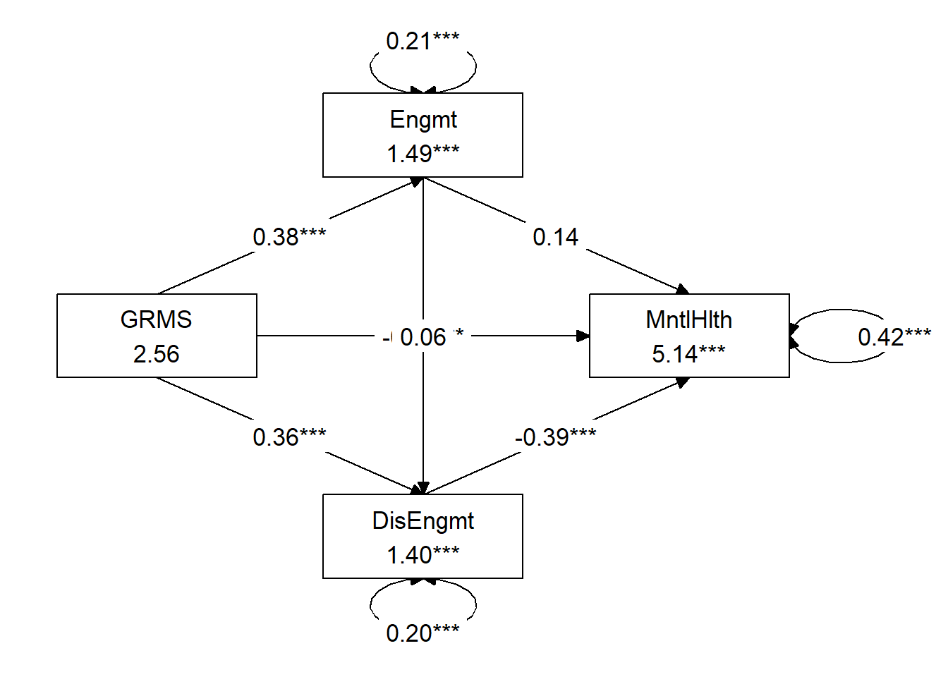
Now let’s make a table.
Table 4
| Model Coefficients Assessing Engagement and Disengagement Coping in a Model of Serial Mediation Predicting Mental Health from Gendered Racial Microaggressions |
|---|
| Predictor | \(B\) | \(SE_{B}\) | \(p\) | \(R^2\) |
|---|
| Engagement coping (M1) | .27 | |||
|---|---|---|---|---|
| Constant | 1.494 | 0.111 | <0.001 | |
| GRMS (\(a_1\)) | 0.384 | 0.042 | <0.001 |
| Disengagement coping (M2) | .29 | |||
|---|---|---|---|---|
| Constant | 1.400 | 0.128 | <0.001 | |
| GRMS (\(a_2\)) | 0.363 | 0.046 | <0.001 | |
| Engagement (\(d_{21}\)) | 0.061 | 0.059 | 0.304 |
| Mental Health (DV) | .37 | |||
|---|---|---|---|---|
| Constant | 5.141 | 0.226 | <0.001 | |
| Engagement (\(b_1\)) | 0.144 | 0.089 | 0.106 | |
| Disengagement (\(b_2\)) | -0.391 | 0.089 | <0.001 | |
| GRMS (\(c'\)) | -0.535 | 0.076 | <0.001 |
| Effects | \(B\) | \(SE_{B}\) | \(p\) | 95% CI |
|---|---|---|---|---|
| Total effect | -0.631 | 0.059 | <0.001 | -0.739, -0.505 |
| Indirect 1 (\(a_1\) * \(a_2\)) | 0.055 | 0.036 | 0.121 | -0.003, 0.140 |
| Indirect 2 (\(b_1\) * \(b_2\)) | -0.142 | 0.038 | <0.001 | -0.227, -0.078 |
| Indirect 3 (\(b_1\) * \(d_{21}\) * \(b_2\)) | -0.009 | 0.009 | 0.339 | -0.032, 0.007 |
| Total indirects | -0.096 | 0.051 | 0.059 | -0.193, 0.007 |
| Contrast1 (Ind1 - Ind2) | 0.197 | 0.053 | <0.001 | 0.106, 0.318 |
| Contrast2 (Ind1 - Ind3) | 0.064 | 0.039 | 0.095 | 0.002, 0.156 |
| Contrast3 (Ind2 - Ind3) | -0.133 | 0.039 | 0.001 | -0.230, -0.066 |
| Note. GRMS = gendered racial microaggressions. The significance of the indirect effects was calculated with bootstrapped, bias-corrected, confidence intervals (.95). |
Working through the data, we should be able to find these items:
- The model accounts for 37% of the variance in predicting mental health outcomes.
- The total effect of GRMS (X) on mental health (Y) is \(-0.631, (p < .001)\); it is negative and statistically significant.
- The direct effect of GRMS (X) on mental health (Y) (\(-0.535, p < 0.001\)) is still negative. Although someone lower in magnitute, it is still statistically significant. While inconsistent with the Baron and Kenny (1986) logic of mediation, Hayes (Hayes, 2022b) argues that a statistically significant indirect effect can stand on its own.
- Indirect effect #1 (\(a_{1}\) x \(b_{1}\) or GRMS through engagement coping to mental health) is \(B = 0.055, p =0.121\). As in the parallel mediation, \(p\) is > .05 and the 95% CIs pass through zero \((-0.003, 0.140)\). Examining the individual paths, there is a statistically significant relationship from GRMS to engagement, but not from engagement to mental health.
- Indirect effect #2 (\(a_{2}\) x \(b_{2}\), or GRMS through disengagement coping to mental health, is \(B = -0.142, p < 0.001, 95CI (-0.227, -0.078)\). Each of the paths is statistically significant from zero and so is the indirect effect.
- Indirect effect #3 (\(a_{2}\) x \(d_{21}\) x \(b_{2}\); GRMS through engagement coping through disengagement coping to mental health) is \(B = -0.009, p = 0.339, 95CI (-0.032, 0.007)\). This indirect effect involves \(a_{1}\) (GRMS to engagement) and \(b_{2}\) which are significant. However, the path from engagement coping to disengagement coping is not significant.
- Total indirect: \(B = -0.096, p = 0.059\) is the sum of all specific indirect effects and is not statistically significant. The positive and negative indirects likely cancel each other out.
- With contrasts we ask: Are the indirect effects statistically significantly different from each other?
- Contrast 1 (indirect 1 v 2): \(B = 0.197, p <0.001)\), yes
- Contrast 2 (indirect 1 v 3): \(B = 0.064, p = 0.095\), no
- Contrast 3 (indirect 2 v 3): \(B = -0.133,p = 0.001p\), yes
- This formal test of contrasts is an important one. It is not ok to infer that effects are statistically significantly different than each other on the basis of their estimates or \(p\) values. The formal test allows us to claim (with justification) that there are statistically significant differences between indirect effects 1 and 2; and 2 and 3.
6.5.3 APA Style Writeup
Method
Data Analysis Serial multiple mediation is appropriate when testing the influence of an independent variable (X) on the dependent variable (Y) directly, as well as indirectly through two or more mediators (M) and there is reason to hypothesize that variables that are causally prior in the model affect all variables later in the causal sequence (Hayes, 2022b). We utilized serial multiple mediation analysis to test the influence of gendered racial microaggressions (X, GRMS) on mental health (Y, MntlHlth) directly as well as indirectly through the mediators engagement coping (M1, Engmt) and disengagement coping (M2, DisEngmt). Moreover, we hypothesized a causal linkage between from the engagement coping mediator to the disengagement coping mediator such that a third specific indirect effect began with GRMS (X) through engagement coping (M1) through disengagement coping (M2) to mental health (Y). Using the lavaan (v. 0.6-16) package in R we followed the procedures outlined in Hayes (2022b) by analyzing the strength and significance of four sets of effects: specific indirect, the total indirect, the direct, and total. Bootstrap analysis, a nonparametric sampling procedure, was used to test the significance of the indirect effects.
Hayes would likely recommend that we say this with fewer acronyms and more words/story.
Results Preliminary Analyses Descriptive statistics were computed, and all variables were assessed univariate normality. You would give your results regarding skew, kurtosis, Shapiro Wilks’, here. If relevant, you could also describe multivariate normality. A summary of descriptive statistics and a correlation matrix for the study is provided in Table 1. These bivariate relations provide evidence to support the test of mediation analysis.
Serial Multiple Mediation Analysis A model of serial multiple mediation was analyzed examining the degree to which engagement and disengagement coping mediated the relationship between gendered racial microaggressions and mental health outcomes. Hayes (2022b) recommended this strategy over simple mediation models because it allows for all mediators to be examined, simultaneously and allows the testing of the seriated effect of prior mediators onto subsequent ones. Using the lavaan (v. 0.6-16) package in R, coefficients for specific indirect, total indirect, direct, and total were computed. Path coefficients refer to regression weights, or slopes, of the expected changes in the dependent variable given a unit change in the independent variables.
Results (depicted in Figure # and presented in Table #) suggest that 37% of the variance in behavioral intentions is accounted for by the three variables in the model. Two of the specific indirect effects were significant and were statistically significantly different from each other. Specifically, the effect of gendered racial microaggressions through disengagement coping to mental health (\(B= -0.142, SE = 0.038, p < .001, 95CI[-0.227, -0.078]\)) was stronger than the indirect effect from gendered racial microaggressions through engagement coping through disengagement coping to mental health (\(B = 0.055, SE = 0.036, p =0.121, 95CI [-0.003, 0.140]\)). Interpreting the results suggests that, mental health outcomes are negatively impacted by gendered racial microaggressions direct and indirectly through disengagement coping. It is this latter path that has the greatest impact.
Note: In a manner consistent with the Lewis et al. (2017) article, the APA Results section can be fairly short. This is especially true when a well-organized table presents the results. In fact, I oculd have left all the numbers out of this except for the \(R^2\) (because it was not reported in the table).
6.6 STAY TUNED
A section on power analysis is planned and coming soon! My apologies that it’s not quite Ready.
6.7 Troubleshooting and FAQs
An indirect effect that was (seemingly) significant in a simple (single) mediation disappears when additional mediators are added.
- Correlated mediators (e.g., multicollinearity) is a likely possibility.
- Which is correct? Maybe both…
A total effect was not significant, but there is one or more statistically significant specific indirect effect
- Recall that a total effect equals the sum of direct and indirect effects. If one specific indirect effect is positive and another is negative, this could account for the NS total effect.
- If the direct effect is NS, but the indirect effects are significant, this might render the total effect NS.
- The indirect effects might operate differently in subpopulations (males, females).
Your editor/peer reviewer/dissertation chair-or-committee member may insist that you do this the Baron & Kenny way (aka “the causal steps approach”).
- Hayes (Hayes, 2022a) provides compelling arguments for how to justify your (I believe correct) decision to just use the PROCESS (aka, bootstrapped, bias corrected, CIs )approach.
- My favorite line in his text reads, ” (the Baron and Kenny way)…is still being taught and recommended by researchers who don’t follow the methodology literature.”
How can I extend a mediation (only) model to include multiple Xs, Ys, or COVs?
- There is fabulous, fabulous narration and syntax for doing all of this in Hayes text. Of course his mechanics are in PROCESS, but lavaan is easy to use by just “drawing more paths” via the syntax. We’ll get more practice as we go along.
What about effect sizes? Shouldn’t we be including/reporting them?
- Yes! The closest thing we have reported to an effect size is \(R^2\), which assess proportion of variance accounted for in the M and Y variables.
- In PROCESS and path analysis this is still emerging. Hayes chapter 4 presents a handful of options for effect sizes beyond \(R^2\).
6.8 Practice Problems
The three problems described below are designed to be grow in this series of chapters that begins with simple mediation and progresses through complex mediation, moderated moderation, and conditional process analysis. The goal of this assignment is to conduct a complex (e.g., parallel or serial) mediation.
I recommend that you select a dataset that includes at least four variables. If you are new to this topic, you may wish to select variables that are all continuously scaled. The IV and moderator (in subsequent chapters) could be categorical (if they are dichotomous, please use 0/1 coding; if they have more than one category it is best if they are ordered). You will likely encounter challenges that were not covered in this chapter. Search for and try out solutions, knowing that there are multiple paths through the analysis.
The suggested practice problem for this chapter is to conduct a parallel or serial mediation (or both).
6.8.1 Problem #1: Rework the research vignette as demonstrated, but change the random seed
If conducting a parallel or serial mediation feels a bit overwhelming, simply change the random seed in the data simulation, then rework one of the chapter problems (i.e., parallel or serial mediation). This should provide minor changes to the data (maybe in the second or third decimal point), but the results will likely be very similar.
6.8.2 Problem #2: Rework the research vignette, but swap one or more variables
Conduct the complex mediation (parallel or serial) using the simulated data provided in this chapter, but swap out one or more of the variables. This could mean changing roles for the variables that were the focus of the chapter, or substituting one or more variables for those in the simulated data but not modeled in the chapter.
6.8.3 Problem #3: Use other data that is available to you
To conduct the parallel or serial mediation, use data for which you have permission and access. This could be IRB approved data you have collected or from your lab; data you simulate from a published article; data from an open science repository; or data from other chapters (or the “homeworked example”) in this OER.
6.8.4 Grading Rubric
| Assignment Component | ||
|---|---|---|
| 1. Assign each variable to the X, Y, M1, and M2 roles | 5 | _____ |
| 4. Use tidySEM to create a figure that represents your results | 5 | _____ |
| 5. Create a table that includes a summary of the effects (indirect, direct, total, total indirect) as well as contrasts | 5 | _____ |
| 6. Represent your work in an APA-style write-up | 5 | _____ |
| 7. Explanation to grader | 5 | _____ |
| 8. Be able to hand-calculate the indirect, direct, and total effects from the a, b, & c’ paths | 5 | _____ |
| Totals | 40 | _____ |
6.9 Homeworked Example
For more information about the data used in this homeworked example, please refer to the description and codebook located at the end of the introductory lesson in ReCentering Psych Stats. An .rds file which holds the data is located in the Worked Examples folder at the GitHub site the hosts the OER. The file name is ReC.rds.
The suggested practice problem for this chapter is to conduct a complex (i.e., parallel or serial) mediation.
Assign each variable to the X, Y, M1, and M2 roles
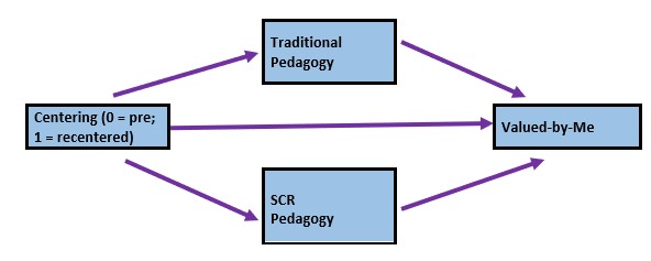
X = Centering: explicit recentering (0 = precentered; 1 = recentered) M1 = TradPed: traditional pedagogy (continuously scaled with higher scores being more favorable) M2 = SRPed: socially responsive pedagogy (continuously scaled with higher scores being more favorable) Y = Valued: valued by me (continuously scaled with higher scores being more favorable)
In this parallel mediation, I am hypothesizing that the perceived course value to the students is predicted by intentional recentering through their assessments of traditional and socially responsive pedagogy.
It helps me to make a quick sketch:
Import the data and format the variables in the model
The approach we are taking to complex mediation does not allow dependency in the data. Therefore, we will include only those who took the multivariate class (i.e., excluding responses for the ANOVA and psychometrics courses).
I need to score the TradPed, SRPed, and Valued variables
TradPed_vars <- c("ClearResponsibilities", "EffectiveAnswers", "Feedback",
    "ClearOrganization", "ClearPresentation")
raw$TradPed <- sjstats::mean_n(raw[, ..TradPed_vars], 0.75)

Valued_vars <- c("ValObjectives", "IncrUnderstanding", "IncrInterest")
raw$Valued <- sjstats::mean_n(raw[, ..Valued_vars], 0.75)

SRPed_vars <- c("InclusvClassrm", "EquitableEval", "MultPerspectives",
    "DEIintegration")
raw$SRPed <- sjstats::mean_n(raw[, ..SRPed_vars], 0.75)
I will create a babydf.
Let’s check the structure of the variables:
## Classes 'data.table' and 'data.frame':   84 obs. of  4 variables:
##  $ Centering: Factor w/ 2 levels "Pre","Re": 2 2 2 2 2 2 2 2 2 2 ...
##  $ TradPed  : num  3.8 5 4.8 4 4.2 3 5 4.6 4 4.8 ...
##  $ Valued   : num  4.33 5 4.67 3.33 4 3.67 5 4 4.67 4.67 ...
##  $ SRPed    : num  4.5 5 5 5 4.75 4.5 5 4.5 5 5 ...
##  - attr(*, ".internal.selfref")=<externalptr>
At this point, these my only inclusion/exclusion criteria. I can determine how many students (who consented) completed any portion of the survey.
Specify and run the lavaan model
ReCpMed <- "
          Valued ~ b1*TradPed + b2*SRPed + c_p*Centering
          TradPed ~ a1*Centering
          SRPed ~ a2*Centering

          indirect1 := a1 * b1
          indirect2 := a2 * b2
          contrast := indirect1 - indirect2
          total_indirects := indirect1 + indirect2
          total_c    := c_p + (indirect1) + (indirect2)
          direct := c_p

          "

set.seed(230916)  #needed for reproducible results since lavaan includes randomness in its estimates
ReCpMedfit <- lavaan::sem(ReCpMed, data = babydf, se = "bootstrap", missing = "fiml")
ReCpMedsummary <- lavaan::summary(ReCpMedfit, standardized = T, rsq = T,
    fit = TRUE, ci = TRUE)
ReC_pMedParamEsts <- lavaan::parameterEstimates(ReCpMedfit, boot.ci.type = "bca.simple",
    standardized = TRUE)
ReCpMedsummary
## lavaan 0.6.17 ended normally after 23 iterations
##
## Estimator ML
## Optimization method NLMINB
## Number of model parameters 11
##
## Number of observations 84
## Number of missing patterns 3
##
## Model Test User Model:
##
## Test statistic 54.059
## Degrees of freedom 1
## P-value (Chi-square) 0.000
##
## Model Test Baseline Model:
##
## Test statistic 145.642
## Degrees of freedom 6
## P-value 0.000
##
## User Model versus Baseline Model:
##
## Comparative Fit Index (CFI) 0.620
## Tucker-Lewis Index (TLI) -1.280
##
## Robust Comparative Fit Index (CFI) 0.613
## Robust Tucker-Lewis Index (TLI) -1.323
##
## Loglikelihood and Information Criteria:
##
## Loglikelihood user model (H0) -202.536
## Loglikelihood unrestricted model (H1) -175.506
##
## Akaike (AIC) 427.071
## Bayesian (BIC) 453.810
## Sample-size adjusted Bayesian (SABIC) 419.110
##
## Root Mean Square Error of Approximation:
##
## RMSEA 0.795
## 90 Percent confidence interval - lower 0.623
## 90 Percent confidence interval - upper 0.982
## P-value H_0: RMSEA <= 0.050 0.000
## P-value H_0: RMSEA >= 0.080 1.000
##
## Robust RMSEA 0.815
## 90 Percent confidence interval - lower 0.641
## 90 Percent confidence interval - upper 1.004
## P-value H_0: Robust RMSEA <= 0.050 0.000
## P-value H_0: Robust RMSEA >= 0.080 1.000
##
## Standardized Root Mean Square Residual:
##
## SRMR 0.217
##
## Parameter Estimates:
##
## Standard errors Bootstrap
## Number of requested bootstrap draws 1000
## Number of successful bootstrap draws 1000
##
## Regressions:
## Estimate Std.Err z-value P(>|z|) ci.lower ci.upper
## Valued ~
## TradPed (b1) 0.686 0.131 5.217 0.000 0.451 0.955
## SRPed (b2) 0.119 0.146 0.816 0.414 -0.193 0.400
## Centerng (c_p) 0.015 0.103 0.143 0.886 -0.182 0.230
## TradPed ~
## Centerng (a1) 0.312 0.137 2.283 0.022 0.047 0.582
## SRPed ~
## Centerng (a2) 0.353 0.113 3.124 0.002 0.130 0.569
## Std.lv Std.all
##
## 0.686 0.747
## 0.119 0.104
## 0.015 0.011
##
## 0.312 0.210
##
## 0.353 0.296
##
## Intercepts:
## Estimate Std.Err z-value P(>|z|) ci.lower ci.upper
## .Valued 0.710 0.469 1.514 0.130 -0.177 1.664
## .TradPed 3.870 0.231 16.773 0.000 3.419 4.291
## .SRPed 4.029 0.186 21.617 0.000 3.675 4.396
## Std.lv Std.all
## 0.710 1.077
## 3.870 5.396
## 4.029 7.013
##
## Variances:
## Estimate Std.Err z-value P(>|z|) ci.lower ci.upper
## .Valued 0.181 0.027 6.658 0.000 0.118 0.224
## .TradPed 0.492 0.128 3.837 0.000 0.259 0.733
## .SRPed 0.301 0.060 5.007 0.000 0.193 0.425
## Std.lv Std.all
## 0.181 0.418
## 0.492 0.956
## 0.301 0.912
##
## R-Square:
## Estimate
## Valued 0.582
## TradPed 0.044
## SRPed 0.088
##
## Defined Parameters:
## Estimate Std.Err z-value P(>|z|) ci.lower ci.upper
## indirect1 0.214 0.105 2.045 0.041 0.032 0.442
## indirect2 0.042 0.053 0.790 0.429 -0.080 0.148
## contrast 0.172 0.125 1.373 0.170 -0.024 0.469
## total_indircts 0.256 0.109 2.346 0.019 0.051 0.469
## total_c 0.271 0.142 1.914 0.056 0.003 0.576
## direct 0.015 0.103 0.143 0.887 -0.182 0.230
## Std.lv Std.all
## 0.214 0.157
## 0.042 0.031
## 0.172 0.126
## 0.256 0.188
## 0.271 0.199
## 0.015 0.011## lhs op rhs label est se
## 1 Valued ~ TradPed b1 0.686 0.131
## 2 Valued ~ SRPed b2 0.119 0.146
## 3 Valued ~ Centering c_p 0.015 0.103
## 4 TradPed ~ Centering a1 0.312 0.137
## 5 SRPed ~ Centering a2 0.353 0.113
## 6 Valued ~~ Valued 0.181 0.027
## 7 TradPed ~~ TradPed 0.492 0.128
## 8 SRPed ~~ SRPed 0.301 0.060
## 9 Centering ~~ Centering 0.233 0.000
## 10 Valued ~1 0.710 0.469
## 11 TradPed ~1 3.870 0.231
## 12 SRPed ~1 4.029 0.186
## 13 Centering ~1 1.369 0.000
## 14 indirect1 := a1*b1 indirect1 0.214 0.105
## 15 indirect2 := a2*b2 indirect2 0.042 0.053
## 16 contrast := indirect1-indirect2 contrast 0.172 0.125
## 17 total_indirects := indirect1+indirect2 total_indirects 0.256 0.109
## 18 total_c := c_p+(indirect1)+(indirect2) total_c 0.271 0.142
## 19 direct := c_p direct 0.015 0.103
## z pvalue ci.lower ci.upper std.lv std.all std.nox
## 1 5.217 0.000 0.415 0.918 0.686 0.747 0.747
## 2 0.816 0.414 -0.161 0.434 0.119 0.104 0.104
## 3 0.143 0.886 -0.194 0.207 0.015 0.011 0.022
## 4 2.283 0.022 0.047 0.582 0.312 0.210 0.435
## 5 3.124 0.002 0.134 0.571 0.353 0.296 0.614
## 6 6.658 0.000 0.143 0.268 0.181 0.418 0.418
## 7 3.837 0.000 0.279 0.813 0.492 0.956 0.956
## 8 5.007 0.000 0.204 0.454 0.301 0.912 0.912
## 9 NA NA 0.233 0.233 0.233 1.000 0.233
## 10 1.514 0.130 -0.109 1.770 0.710 1.077 1.077
## 11 16.773 0.000 3.383 4.286 3.870 5.396 5.396
## 12 21.617 0.000 3.666 4.382 4.029 7.013 7.013
## 13 NA NA 1.369 1.369 1.369 2.837 1.369
## 14 2.045 0.041 0.034 0.451 0.214 0.157 0.325
## 15 0.790 0.429 -0.044 0.174 0.042 0.031 0.064
## 16 1.373 0.170 -0.026 0.456 0.172 0.126 0.261
## 17 2.346 0.019 0.053 0.472 0.256 0.188 0.389
## 18 1.914 0.056 0.003 0.577 0.271 0.199 0.411
## 19 0.143 0.887 -0.194 0.207 0.015 0.011 0.022Use tidySEM to create a figure that represents your results
# only worked when I used the library to turn on all these pkgs
library(lavaan)
library(dplyr)
library(ggplot2)
library(tidySEM)
tidySEM::graph_sem(model = ReCpMedfit)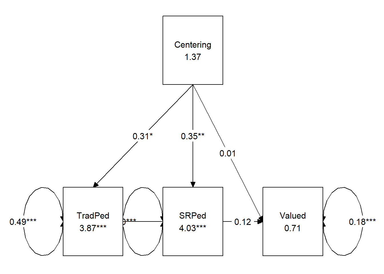
##      [,1]      [,2]        [,3]
## [1,] NA        "Centering" NA
## [2,] "TradPed" "SRPed"     "Valued"
## attr(,"class")
## [1] "layout_matrix" "matrix"        "array"
To create the figure I showed at the beginning of the chapter, we will want three rows and three columns.
ReCpMed_map <- tidySEM::get_layout("", "TradPed", "", "Centering", "",
    "Valued", "", "SRPed", "", rows = 3)
ReCpMed_map
## [,1] [,2] [,3]
## [1,] "" "TradPed" ""
## [2,] "Centering" "" "Valued"
## [3,] "" "SRPed" ""
## attr(,"class")
## [1] "layout_matrix" "matrix" "array"tidySEM::graph_sem(ReCpMedfit, layout = ReCpMed_map, rect_width = 1.5,
rect_height = 1.25, spacing_x = 2, spacing_y = 3, text_size = 4.5)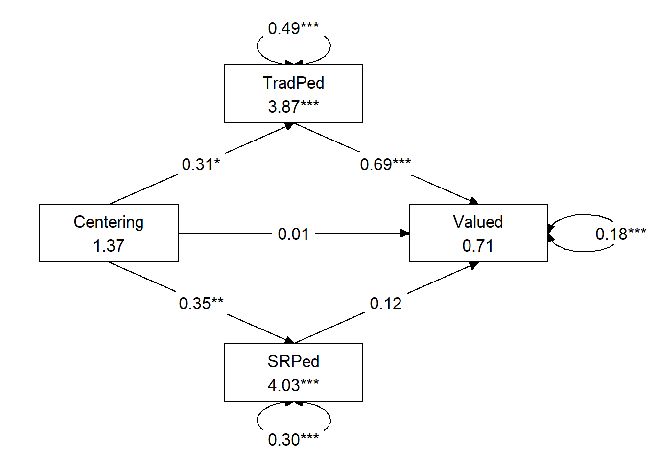
Create a table that includes a summary of the effects (indirect, direct, total, total indirect) as well as contrasts
I will write my results to a .csv file.
Table 1
| Model Coefficients Assessing Students’ Appraisal of Traditional and Socially Responsive Pedagogy in a Model of Parallel Mediation Predicting Perceived Course Value from Explicit Recentering |
|---|
| Predictor | \(B\) | \(SE_{B}\) | \(p\) | \(R^2\) |
|---|
| Traditional Pedagogy (M1) | .04 | |||
|---|---|---|---|---|
| Constant | 3.870 | 0.231 | <0.001 | |
| Centering (\(a_1\)) | 0.312 | 0.137 | 0.022 |
| Socially Responsive Pedagogy (M2) | .09 | |||
|---|---|---|---|---|
| Constant | 4.029 | 0.186 | <0.001 | |
| Centering (\(a_2\)) | 0.353 | 0.113 | 0.002 |
| Perceived Course Value (DV) | .58 | |||
|---|---|---|---|---|
| Constant | 0.710 | 0.469 | 0.130 | |
| Traditional Pedagogy (\(b_1\)) | 0.686 | 0.131 | <0.001 | |
| Socially Rx Pedagogy (\(b_2\)) | 0.119 | 0.146 | 0.414 | |
| Centering (\(c'\)) | 0.015 | 0.103 | 0.886 |
| Effects | \(B\) | \(SE_{B}\) | \(p\) | 95% CI |
|---|---|---|---|---|
| Total effect | 0.271 | 0.142 | 0.056 | 0.003, 0.577 |
| Indirect 1 (\(a_1\) * \(b_1\)) | 0.214 | 0.105 | 0.041 | 0.034, 0.451 |
| Indirect 2 (\(a_2\) * \(b_2\)) | 0.042 | 0.053 | 0.429 | -0.044, 0.174 |
| Total indirects | 0.256 | 0.109 | 0.019 | 0.053, 0.472 |
| Contrast1 (Ind1 - Ind2) | 0.172 | 0.125 | 0.170 | -0.026, 0.456 |
| Note. The significance of the indirect effects was calculated with bootstrapped, bias-corrected, confidence intervals (.95). |
Represent your work in an APA-style write-up
A model of parallel mediation analyzed the degree to which students’ perceptions of traditional and socially responsive pedagogy mediated the relationship between explicit recentering of the course and course value. Hayes (2022b) recommended this strategy over simple mediation models because it allows for all mediators to be examined, simultaneously. The resultant direct and indirect values for each path account for other mediation paths. Using the lavaan (v. 0.6-16) package in R, coefficients for specific indirect, total indirect, direct, and total were computed. Path coefficients refer to regression weights, or slopes, of the expected changes in the dependent variable given a unit change in the independent variables.
Results (depicted in Figure 1 and presented in Table 1) suggest that 58% of the variance in perceptions of course value is accounted for by the model. The indirect effect predicting course value from explicit recentering through traditional pedagogy was statistically significant \((B = 0.214, SE = 0.105, p = 0.041, 95CI [0.034, 0.451])\). Examining the individual paths we see that \(a_{1}\) was positive and statistically significant (recentering is associated with higher evaluations of traditional pedagogy). The \(b_{1}\) path was similarly statistically significant (traditional pedagogy was associated with course valuation). The indirect effect predicting course value from recentering through socially responsive pedagogy was not statistically significant \(B = 0.042, SE = 0.053, p = 0.429, 95CE[-0.044, 0.174])\). While explicit recentering had a statistically significant effect on ratings of socially responsive pedagogy (i.e., the \(a_{2}\) path), socially responsive pedagogy did not have a statistically significant effect on perceptions of course value (i.e., the \(b_{2}\) path). The drop in magnitude and near-significance from the total effect \((B = 0.271, p = 0.056)\) to the direct effect \((B = 0.015, p = 0.886)\) supports the presence of mediation. A pairwise comparison of the specific indirect effects indicated that the strength of the effects were not statistically significantly different from each other. In summary, the effects of explicit recentering on perceived value to the student appears to be mediated through students evaluation of traditional pedagogy.