Chapter 5 Simple Mediation
The focus of this lecture is to estimate indirect effects (aka “mediation”). We examine the logic/design required to support the argument that mediation is the mechanism that explains the X –> Y relationship. We also work three examples (one with covariates).
At the outset, please note that although I rely heavily on Hayes (2018) text and materials, I am using the R package lavaan in these chapters. In recent years, Hayes has introduced a PROCESS macro for R. Because I am not yet up-to-speed on using this macro (it is not a typical R package) and because ReCentering Psych Stats uses lavaan for confirmatory factor analysis and structural equation modeling, I have chosen to utilize the lavaan package. A substantial difference is that the PROCESS macros use ordinary least squares and lavaan uses maximum likelihood estimators.
5.2 Estimating Indirect Effects (the analytic approach often termed mediation)
5.2.1 The definitional and conceptual
As in Hayes text (2018), we will differentiate between moderation and mediation. Conditional process analysis involves both! With each of these, we are seeking to understand the mechanism at work that leads to the relationship (be it correlational, predictive, or causal)
Even though this process has sometimes been termed causal modeling, Hayes argues that his statistical approach is not claiming to determine cause; that is really left to the argument of the research design.
Moderation (a review):
- Answers questions of when or for whom and is often the source of the answer, it depends.
- Think of our interaction effects in ANOVA and regression
- The effect of X on some variable Y is moderated by W if its size, sign, or strength depends on, or can be predicted, by W. Then we can say, “W is a moderator of X’s effect on Y” or “W and X interact in their influence on Y.”
- The image below illustrates moderation with conceptual and statistical diagrams. Note that three predictors (IV, DV, their interaction) point to the DV.
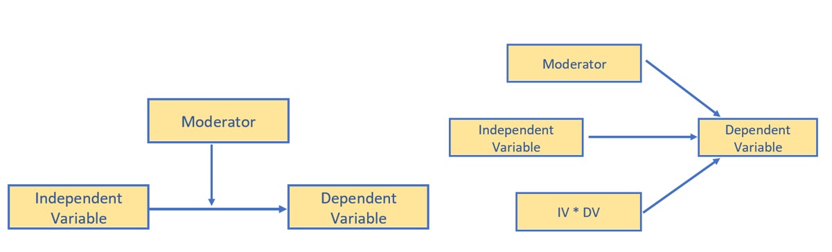
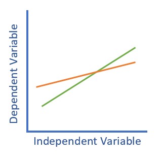
The classic plot of moderation results is often the best way to detect that an interaction was included in the analysis and helps understand the conditional (e.g., for whom, under what conditions) nature of the analysis.
Mediation:
- Answers questions of how (I also think through and via to describe the proposed mediating mechanism)
- Paths in a mediation model are direct (X does not pass through M on its way to Y) and indirect (X passes through M on its way to Y). Once we get into the statistics, we will also be focused on total effects.
- Hayes thinks in terms of antecedent and consequent variables. In a 3-variable, simple mediation, X and M are the antecedent variables; X and M are the consequent variables.
- There is substantial debate and controversy about whether we can say “the effect of X on Y is mediated through M” or whether we should say, “There is a statistically significant indirect effect of X on Y thru M.” Hayes comes down on the “use mediation language” side of the debate.
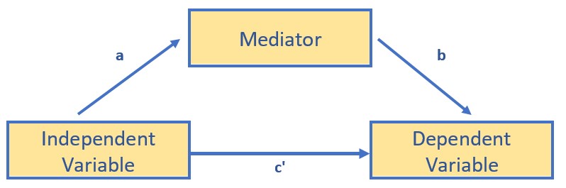
- In sum, a simple mediation model is any causal system in which at least one causal antecedent X variable is proposed as influencing an outcome Y through a single intervening variable, M. In such a model there are two pathways by which X can influence Y.
- The figure below doubles as both the conceptual and statistical diagram of evaluating a simple mediation – a simple indirect effect.
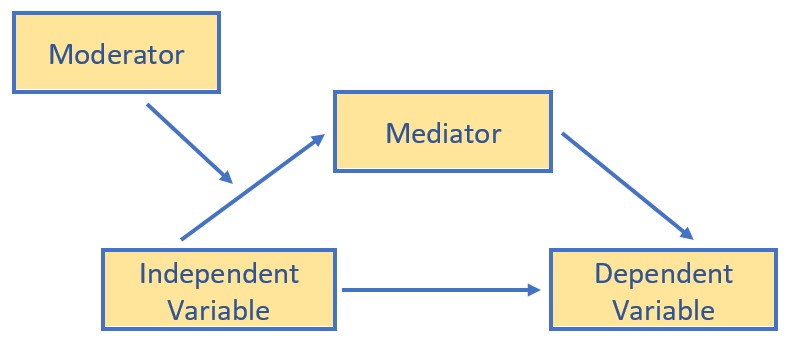
Conditional process analysis:
- Used when the research goal is to understand the boundary conditions of the mechanism(s) by which a variable transmits its effect on another.
- Typically, simultaneously, assesses the influence of mediating (indirect effects) and moderating (interactional effects) in a model-building fashion.
- In a conditional process model, the moderator(s) may be hypothesized to influence one or more of the paths.
We will work toward building a conditional process model, a moderated mediation, over the next several chapters.
5.3 Workflow for Simple Mediation
The following is a proposed workflow for conducting a simple mediation.
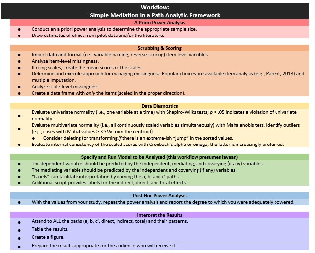
Conducting a simple mediation involves the following steps:
- Conducting an a priori power analysis to determine the appropriate sample size.
- This will require estimates of effect that are drawn from pilot data, the literature, or both.
- Scrubbing and scoring the data.
- Guidelines for such are presented in the respective lessons.
- Conducting data diagnostics, this includes:
- item and scale level missingness,
- internal consistency coefficients (e.g., alphas or omegas) for scale scores,
- univariate and multivariate normality
- Specifying and running the model (this lesson presumes it will with the R package, lavaan).
- The dependent variable should be predicted by the independent, mediating, and covarying (if any) variables.
- “Labels” can facilitate interpretation by naming the a, b, and c’ paths. +Additional script provides labels for the indirect, direct, and total effects.
- Conducting a post hoc power analysis.
- Informed by your own results, you can see if you were adequately powered to detect a statistically significant effect, if, in fact, one exists.
- Interpret and report the results.
- Interpret ALL the paths and their patterns.
- Create a table and figure.
- Prepare the results in a manner that is useful to your audience.
In addition to the workflow through the statistical problem, the very traditional and classic figure below is useful in understanding the logic beneath mediation as the explanatory mechanism.
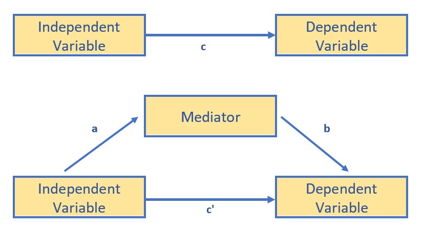
The top figure represents the bivariate relationship between the independent and dependent variable. The result of a simple linear regression (one predictor) represent the total effect of the IV on the DV. We can calculate this by simply regressing the DV onto the IV. The resulting \(B\) weight is known as the c path. A bivariate correlation coefficient results in the same value – only it is standardized (so would be the same as the \(\beta\) weight).
The lower figure represents that the relationship between the IV and DV is mediated by a third variable. We assign three labels to the paths: a, between the IV and mediator; b, between the mediator and DV; and c’ (c prime) between the IV and DV.
Although Hayes makes a compelling case that we can claim “mediation” when there is a statistically significant indirect effect (2018), traditionally, a mediated relationship is supported when the value of c’ is statistically significantly lower than c. When this occurs, then know that the mediator is sharing some of the variance (and therefore acting as a conduit) in the prediction of the DV.
You might already be imagining potential challenges to this model. For example, which variable should be the IV and which one should be the mediator? Can we switch them? You can – and you will likely have very similar (if not identical) results. Good research design is what provides support for suggesting that mediation is the proper, casual, mechanism regarding the relationship between the IV and DV. An excellent review of the challenges of establishing a robust mediation model is provided by Kline (2015), where he suggests the following as the minimally required elements of a mediation design:
- the IV is an experimental variable with random assignment to conditions;
- the mediator is an individual difference variable that is not manipulated and is measured at a later time;and
- the DV is measured at a third occasion
These criteria are in addition to the rather standard criteria for establishing causality (see Stone-Romero & Rosopa, 2010 for a review):
- temporal precedence,
- statistical covariation, and
- ruling out plausible rival hypotheses.
Some journals take this very seriously. In fact FAQs in the Journal of Vocational Behavior make it clear that they will very rarely publish a “mediation manuscript” unless it has a minimum of three waves.
Working through a mediation will help operationalize these concepts.
5.4 Super Simple Mediation in lavaan: A focus on the mechanics
The lavaan tutorial (Rosseel, 2020) provides a helpful model of how writing code to estimate an indirect effect. Using the lavaan tutorial as our guide, let’s start with just a set of fake data with variable names that represent X (predictor, IV, antecedent), M (mediator, atencedent, consequent), and Y (outcome, DV, consequent).
5.4.1 Simulate Fake Data
The code below is asking to create a dataset with a sample size of 100. The dataset has 3 variables, conveniently named X (predictor, antecedent, IV), M (mediator), and Y (outome, consequent, DV). The R code asks for random selection of numbers with a normal distribution. You can see that the M variable will be related to the X variable by + .5; and the Y variable will be related to the M variable by + .7. This rather ensures a statistically significant indirect effect.
5.4.2 Specify Mediation Model
The package we are using is lavaan. Hayes’ model is path analysis, which can be a form of structural equation modeling. As a quick reminder, in SPSS, PROCESS is limited to ordinary least squares regression. We will use maximum likliehood estimators for the Hayes/PROCESS examples, but lavaan can take us further than PROCESS because
- We can (and, in later chapters, will) do latent variable modeling.
- We can have more specificity and flexibility than the prescribed PROCESS models allow. I say this with all due respect to Hayes – there is also a good deal of flexibility to be able to add multiple mediators and covariates within most of the Hayes’ prescribed models.
Hayes text is still a great place to start because the conceptual and procedural information is clear and transferable to the R environment.
Our atheoretical dataset makes it easy to identify which variable belongs in each role (X,Y,M). When specifying the paths in lavaan, here’s what to keep in mind:
- Name your model/object (below is X, “<-” means “is defined by”)
- The model exists between 2 single quotation marks (the odd looking ’ and ’ at the beginning and end).
- The # of regression equations you need depends on the # of variables that have arrows pointing to them. In a simple mediation, there are 3 variables with 2 variables having arrows pointing to them – need 2 regression equations:
- one for the Mediator
- one for the DV (Y)
- Operator for a regression analysis is the (tilde, ~)
- DV goes on left
- In first equation we regress both the X and M onto Y
- In second equation we regress M onto X
- The asterisk (*) is a handy tool to label variables (don’t confuse it as defining an interaction); this labeling as a, b, and c_p (in traditional mediation, the total effect is labeled with a and the direct effect is c’[c prime], but the script won’t allow and extra single quotation mark, hence c_p) is super helpful in interpreting the ouput
- The indirect effect is created by multiplying the a and b paths.
- The “:=” sign is used when creating a new variable that is a function of variables in the model, but not in the dataset (i.e., the a and b path).
After specifying the model, we create an object that holds our results from the SEM. To obtain all the results from our of indirect effects, we also need to print a summary of the fit statistics, standardized estimates, r-squared, and confidence intervals.
Other authors will write the model code more sensibly, predicting the mediator first, and then the Y variable. However, I found that by doing it this way, the semPlot produces a more sensible figure.
Also, because we set a random seed, you should get the same results, but if it differs a little, don’t panic. Also, in Hayes text the direct path from X to Y is c’ (“c prime”; where as c is reserved for the total effect of X on Y).
Let’s run the whole model.
model <- "
          Y ~ b*M + c_p*X
          M ~ a*X

          indirect :=  a*b
          direct  := c_p
          total_c  := c_p + (a*b)

          "
set.seed(230916)  #needed for reproducibility especially when specifying bootstrapped confidence intervals
fit <- lavaan::sem(model, data = Data, se = "bootstrap", missing = "fiml")
FDsummary <- lavaan::summary(fit, standardized = T, rsq = T, fit = TRUE,
    ci = TRUE)
FD_ParamEsts <- lavaan::parameterEstimates(fit, boot.ci.type = "bca.simple",
    standardized = TRUE)
FDsummary
## lavaan 0.6.17 ended normally after 1 iteration
##
## Estimator ML
## Optimization method NLMINB
## Number of model parameters 7
##
## Number of observations 100
## Number of missing patterns 1
##
## Model Test User Model:
##
## Test statistic 0.000
## Degrees of freedom 0
##
## Model Test Baseline Model:
##
## Test statistic 66.380
## Degrees of freedom 3
## P-value 0.000
##
## User Model versus Baseline Model:
##
## Comparative Fit Index (CFI) 1.000
## Tucker-Lewis Index (TLI) 1.000
##
## Robust Comparative Fit Index (CFI) 1.000
## Robust Tucker-Lewis Index (TLI) 1.000
##
## Loglikelihood and Information Criteria:
##
## Loglikelihood user model (H0) -279.032
## Loglikelihood unrestricted model (H1) -279.032
##
## Akaike (AIC) 572.064
## Bayesian (BIC) 590.301
## Sample-size adjusted Bayesian (SABIC) 568.193
##
## Root Mean Square Error of Approximation:
##
## RMSEA 0.000
## 90 Percent confidence interval - lower 0.000
## 90 Percent confidence interval - upper 0.000
## P-value H_0: RMSEA <= 0.050 NA
## P-value H_0: RMSEA >= 0.080 NA
##
## Robust RMSEA 0.000
## 90 Percent confidence interval - lower 0.000
## 90 Percent confidence interval - upper 0.000
## P-value H_0: Robust RMSEA <= 0.050 NA
## P-value H_0: Robust RMSEA >= 0.080 NA
##
## Standardized Root Mean Square Residual:
##
## SRMR 0.000
##
## Parameter Estimates:
##
## Standard errors Bootstrap
## Number of requested bootstrap draws 1000
## Number of successful bootstrap draws 1000
##
## Regressions:
## Estimate Std.Err z-value P(>|z|) ci.lower ci.upper
## Y ~
## M (b) 0.708 0.085 8.360 0.000 0.537 0.869
## X (c_p) -0.107 0.112 -0.954 0.340 -0.327 0.114
## M ~
## X (a) 0.513 0.097 5.278 0.000 0.334 0.708
## Std.lv Std.all
##
## 0.708 0.639
## -0.107 -0.080
##
## 0.513 0.426
##
## Intercepts:
## Estimate Std.Err z-value P(>|z|) ci.lower ci.upper
## .Y -0.022 0.097 -0.224 0.822 -0.212 0.179
## .M -0.031 0.097 -0.320 0.749 -0.232 0.143
## Std.lv Std.all
## -0.022 -0.018
## -0.031 -0.028
##
## Variances:
## Estimate Std.Err z-value P(>|z|) ci.lower ci.upper
## .Y 0.927 0.127 7.315 0.000 0.669 1.160
## .M 0.981 0.128 7.636 0.000 0.716 1.229
## Std.lv Std.all
## 0.927 0.629
## 0.981 0.818
##
## R-Square:
## Estimate
## Y 0.371
## M 0.182
##
## Defined Parameters:
## Estimate Std.Err z-value P(>|z|) ci.lower ci.upper
## indirect 0.363 0.084 4.328 0.000 0.216 0.543
## direct -0.107 0.112 -0.953 0.340 -0.327 0.114
## total_c 0.257 0.120 2.132 0.033 0.024 0.507
## Std.lv Std.all
## 0.363 0.272
## -0.107 -0.080
## 0.257 0.192## lhs op rhs label est se z pvalue ci.lower ci.upper
## 1 Y ~ M b 0.708 0.085 8.360 0.000 0.541 0.871
## 2 Y ~ X c_p -0.107 0.112 -0.954 0.340 -0.326 0.120
## 3 M ~ X a 0.513 0.097 5.278 0.000 0.332 0.705
## 4 Y ~~ Y 0.927 0.127 7.315 0.000 0.713 1.252
## 5 M ~~ M 0.981 0.128 7.636 0.000 0.766 1.282
## 6 X ~~ X 0.827 0.000 NA NA 0.827 0.827
## 7 Y ~1 -0.022 0.097 -0.224 0.822 -0.218 0.174
## 8 M ~1 -0.031 0.097 -0.320 0.749 -0.210 0.183
## 9 X ~1 -0.005 0.000 NA NA -0.005 -0.005
## 10 indirect := a*b indirect 0.363 0.084 4.328 0.000 0.224 0.557
## 11 direct := c_p direct -0.107 0.112 -0.953 0.340 -0.326 0.120
## 12 total_c := c_p+(a*b) total_c 0.257 0.120 2.132 0.033 0.029 0.517
## std.lv std.all std.nox
## 1 0.708 0.639 0.639
## 2 -0.107 -0.080 -0.088
## 3 0.513 0.426 0.469
## 4 0.927 0.629 0.629
## 5 0.981 0.818 0.818
## 6 0.827 1.000 0.827
## 7 -0.022 -0.018 -0.018
## 8 -0.031 -0.028 -0.028
## 9 -0.005 -0.005 -0.005
## 10 0.363 0.272 0.299
## 11 -0.107 -0.080 -0.088
## 12 0.257 0.192 0.2115.4.3 Interpret the Output
Note that in the script we ask (and get) two sets of parameter estimates. The second set (in the really nice dataframe) includes bootstrapped, bias-corrected confidence intervals. Bias-corrected confidence interals have the advantage of being more powerful and bias-free. Note, though, that when the CI crosses 0, the effect is NS.
So let’s look at this step-by-step.
- Overall, our model accounted for 37% of the variance in the IV and 18% of the variance in the mediator.
- a path = \(B = 0.513, p < 0.001\)
- b path = \(0.708, p < 0.001\)
- the indirect effect is a product of the a and b paths \((0.513 * 0.708 = 0.363)\); while we don’t hand calculate it’s significance, we see that it is \(p < 0.001\).
- the direct effect (c’, c prime, or c_p) is the isolated effect of X on Y when including M as a predictor. We hope this value is lower than the total effect because this means that including M shared some of the variance in predicting Y: \(c' = -0.107, p = 0.340\), and it is no longer significant.
- we also see the total effect; this value is
- identical to the value of simply predicting Y on X (with no M it the model)
- the value of a(b) + c_p: \((0.513 * 0.708) + (-0.107) = 0.257; (p = 0.033)\)
Here’s a demonstration that the total effect is, simply, predicting Y from X:
##
## Call:
## lm(formula = Y ~ X, data = Data)
##
## Residuals:
##      Min       1Q   Median       3Q      Max
## -2.36350 -0.90598 -0.07158  0.74879  2.52079
##
## Coefficients:
##             Estimate Std. Error t value Pr(>|t|)
## (Intercept) -0.04374    0.12035  -0.363   0.7171
## X            0.25668    0.13237   1.939   0.0554 .
## ---
## Signif. codes:  0 '***' 0.001 '**' 0.01 '*' 0.05 '.' 0.1 ' ' 1
##
## Residual standard error: 1.204 on 98 degrees of freedom
## Multiple R-squared:  0.03695,    Adjusted R-squared:  0.02712
## F-statistic:  3.76 on 1 and 98 DF,  p-value: 0.05537
In a simple model such as this, it is also the same value as the bivariate correlation. The only trick is that the bivariate correlation produces a standardized result; so it would be the \(\beta\).
## Call:corr.test(x = Data[c("Y", "X")])
## Correlation matrix
##      Y    X
## Y 1.00 0.19
## X 0.19 1.00
## Sample Size
## [1] 100
## Probability values (Entries above the diagonal are adjusted for multiple tests.)
##      Y    X
## Y 0.00 0.06
## X 0.06 0.00
##
##  To see confidence intervals of the correlations, print with the short=FALSE option
5.4.4 A Figure and Table
We can use the package tidySEM to create a figure that includes the values on the path.
Here’s what the base package gets us
## This is lavaan 0.6-17
## lavaan is FREE software! Please report any bugs.##
## Attaching package: 'lavaan'## The following object is masked from 'package:psych':
##
## cor2cov##
## Attaching package: 'dplyr'## The following objects are masked from 'package:stats':
##
## filter, lag## The following objects are masked from 'package:base':
##
## intersect, setdiff, setequal, union##
## Attaching package: 'ggplot2'## The following objects are masked from 'package:psych':
##
## %+%, alpha## Loading required package: OpenMx##
## Attaching package: 'OpenMx'## The following object is masked from 'package:psych':
##
## tr## Registered S3 method overwritten by 'tidySEM':
## method from
## predict.MxModel OpenMx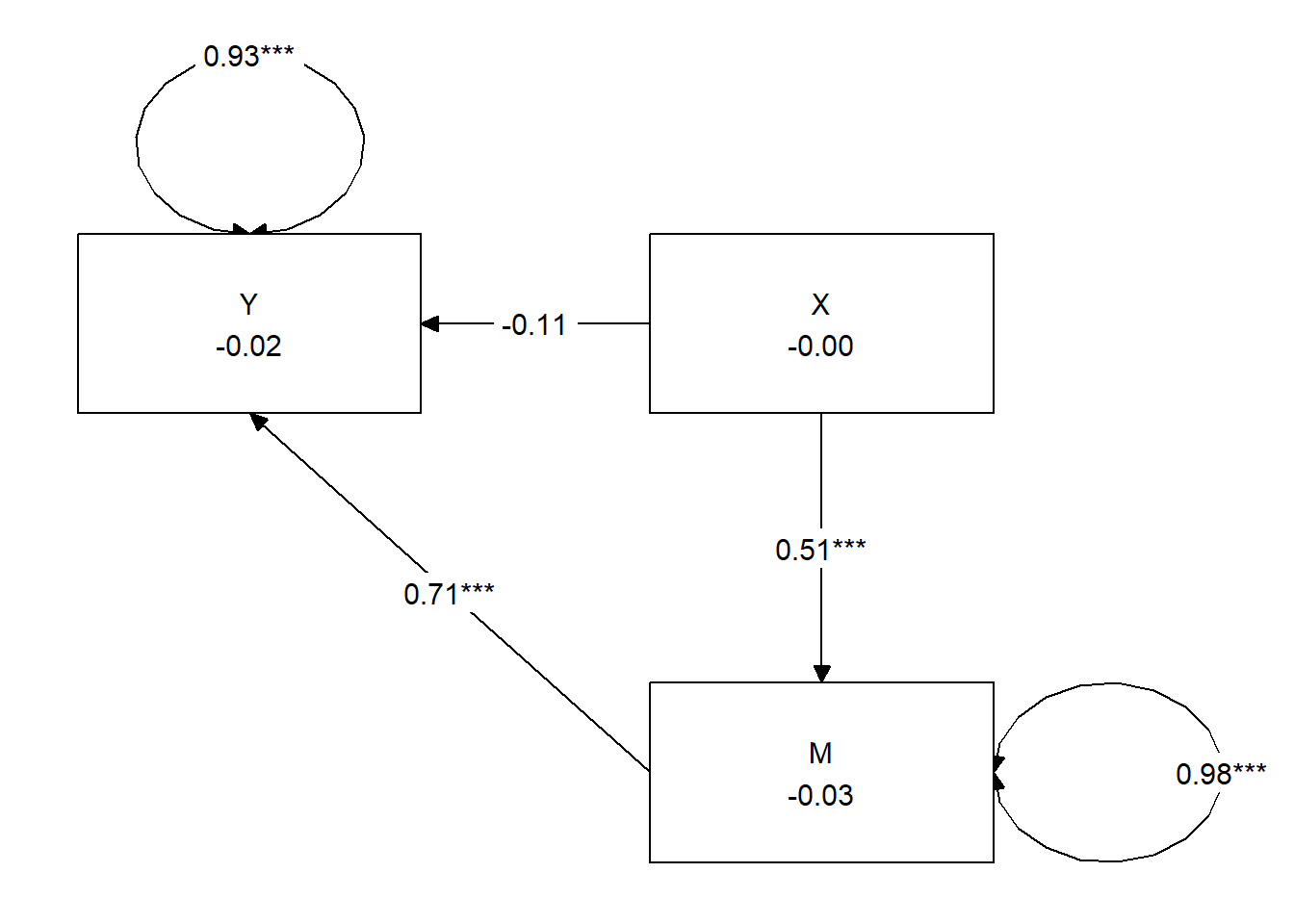 Hayes has great examples of APA style tables that have become the standard way to communicate results. I haven’t yet found a package that will turn this output into a journal-ready table, however with a little tinkering, we can approximate one of the standard tables. This code lets us understand the label names and how they are mapped
## [,1] [,2] [,3]
## [1,] "Y" "M" "X"
## attr(,"class")
## [1] "layout_matrix" "matrix" "array"We can write code to remap them
## [,1] [,2] [,3]
## [1,] "" "M" ""
## [2,] "X" "" "Y"
## attr(,"class")
## [1] "layout_matrix" "matrix" "array"We run again with our map and BOOM! Still needs tinkering for gorgeous, but hey!
tidySEM::graph_sem(fit, layout = med_map, rect_width = 1.5, rect_height = 1.25,
spacing_x = 2, spacing_y = 3, text_size = 4.5) To assist in table preparation, it is possible to export the results to a .csv file that can be manipulated in Excel, Microsoft Word, or other program to prepare an APA style table.
Check with your discipline’s journals to see how results of mediations are reported. Here’s a version that I like.
Table 1
| Model Coefficients Assessing M as a Mediator Between X and Y |
|---|
| Mediator (M) | Dependent Variable (Y) |
| Antecedent | path | \(B\) | \(SE\) | \(p\) | path | \(B\) | \(SE\) | \(p\) |
| constant | \(i_{M}\) | 0.031 | 0.097 | 0.749 | \(i_{Y}\) | -0.022 | 0.097 | 0.822 |
| Independent (X) | \(a\) | 0.513 | 0.097 | < 0.001 | \(c'\) | -0.107 | 0.112 | 0.340 |
| Mediator (M) | \(b\) | 0.708 | 0.085 | < 0.0 |
| \(R^2\) = 18% | \(R^2\) = 37% |
| Note. The value of the indirect effect was \(B = 0.363, SE = 0.084, p < 0.001, 95CI(0.224, 0.557)\) |
5.4.5 Results
A simple mediation model examined the degree to which M mediated the relation of X on Y. Using the lavaan package (v 0.6-16) in R, coefficients for each path, the indirect effect, and total effects were calculated. These values are presented in Table 1 and illustrated in Figure 1. Results suggested that 18% of the variance in M and 37% of the variance in Y were accounted for in the model. The indirect effect (\(B = 0.363, SE = 0.084, p < 0.001\)) was statistically significant; the direct effect (\(B = -0.107, SE = 0.112, p = 0.340\)) was not. Comparing the nonsignificant direct effect to the statistically significant total effect (\(B = 0.257, SE = 0.120, p = 0.033\)) is consistent with the notion that the effect of X on Y is explained through M.
5.5 Research Vignette
The research vignette comes from the Kim, Kendall, and Cheon’s (2017), “Racial Microaggressions, Cultural Mistrust, and Mental Health Outcomes Among Asian American College Students.” Participants were 156 Asian American undergraduate students in the Pacific Northwest. The researchers posited the a priori hypothesis that cultural mistrust would mediate the relationship between racial microaggressions and two sets of outcomes: mental health (e.g., depression, anxiety, well-being) and help-seeking.
Variables used in the study included:
- REMS: Racial and Ethnic Microaggressions Scale (Nadal, 2011). The scale includes 45 items on a 2-point scale where 0 indicates no experience of a microaggressive event and 1 indicates it was experienced at least once within the past six months. Higher scores indicate more experience of microaggressions.
- CMI: Cultural Mistrust Inventory (Terrell & Terrell, 1981). This scale was adapted to assess cultural mistrust harbored among Asian Americans toward individuals from the mainstream U.S. culture (e.g., Whites). The CMI includes 47 items on a 7-point scale where higher scores indicate a higher degree of cultural mistrust.
- ANX, DEP, PWB: Subscales of the Mental Health Inventory (Veit & Ware, 1983) that assess the mental health outcomes of anxiety (9 items), depression (4 items), and psychological well-being (14 items). Higher scores (on a 6 point scale) indicate stronger endorsement of the mental health outcome being assessed.
- HlpSkg: The Attiudes Toward Seeking Professional Psychological Help – Short Form (Fischer & Farina, 1995) includes 10 items on a 4-point scale (0 = disagree, 3 = agree) where higher scores indicate more favorable attitudes toward help seeking.
5.5.1 Data Simulation
We used the lavaan::simulateData function for the simulation. If you have taken psychometrics, you may recognize the code as one that creates latent variables form item-level data. In trying to be as authentic as possible, we retrieved factor loadings from psychometrically oriented articles that evaluated the measures (Nadal, 2011; Veit & Ware, 1983). For all others we specified a factor loading of 0.80. We then approximated the measurement model by specifying the correlations between the latent variable. We sourced these from the correlation matrix from the research vignette (Paul Youngbin Kim et al., 2017). The process created data with multiple decimals and values that exceeded the boundaries of the variables. For example, in all scales there were negative values. Therefore, the final element of the simulation was a linear transformation that rescaled the variables back to the range described in the journal article and rounding the values to integer (i.e., with no decimal places).
# Entering the intercorrelations, means, and standard deviations from
# the journal article
Kim_generating_model <- "
##measurement model
REMS =~ .82*Inf32 + .75*Inf38 + .74*Inf21 + .72*Inf17 + .69*Inf9 + .61*Inf36 + .51*Inf5 + .49*Inf22 + .81*SClass6 + .81*SClass31 + .74*SClass8 + .74*SClass40 + .72*SClass2 + .65*SClass34 + .55*SClass11 + .84*mInv27 + .84*mInv30 + .80*mInv39 + .72*mInv7 + .62*mInv26 + .61*mInv33 + .53*mInv4 + .47*mInv14 + .47*mInv10 + .74*Exot3 + .74*Exot29 + .71*Exot45 + .69*Exot35 + .60*Exot42 + .59*Exot23 + .51*Exot13 + .51*Exot20 + .49*Exot43 + .84*mEnv37 + .85*mEnv24 + .78*mEnv19 + .70*mEnv28 + .69*mEnv18 + .55*mEnv41 + .55*mEnv12 + .76*mWork25 + .67*mWork15 + .65*mWork1 + .64*mWork16 + .62*mWork44
CMI =~ .8*cmi1 + .8*cmi2 + .8*cmi3 + .8*cmi4 + .8*cmi5 + .8*cmi6 + .8*cmi7 + .8*cmi8 + .8*cmi9 + .8*cmi10 + .8*cmi11 + .8*cmi12 + .8*cmi13 + .8*cmi14 + .8*cmi15 + .8*cmi16 + .8*cmi17 + .8*cmi18 + .8*cmi19 + .8*cmi20 + .8*cmi21 + .8*cmi22 + .8*cmi23 + .8*cmi24 + .8*cmi25 + .8*cmi26 + .8*cmi27 + .8*cmi28 + .8*cmi29 + .8*cmi30 + .8*cmi31 + .8*cmi32 + .8*cmi33 + .8*cmi34 + .8*cmi35 + .8*cmi36 + .8*cmi37 + .8*cmi38 + .8*cmi39 + .8*cmi40 + .8*cmi41 + .8*cmi42 + .8*cmi43 + .8*cmi44 + .8*cmi45 + .8*cmi46 + .8*cmi47
ANX =~ .80*Anx1 + .80*Anx2 + .77*Anx3 + .74*Anx4 + .74*Anx5 + .69*Anx6 + .69*Anx7 + .68*Anx8 + .50*Anx9
DEP =~ .74*Dep1 + .83*Dep2 + .82*Dep3 + .74*Dep4
PWB =~ .83*pwb1 + .72*pwb2 + .67*pwb3 + .79*pwb4 + .77*pwb5 + .75*pwb6 + .74*pwb7 +.71*pwb8 +.67*pwb9 +.61*pwb10 +.58*pwb11
HlpSkg =~ .8*hlpskg1 + .8*hlpskg2 + .8*hlpskg3 + .8*hlpskg4 + .8*hlpskg5 + .8*hlpskg6 + .8*hlpskg7 + .8*hlpskg8 + .8*hlpskg9 + .8*hlpskg10
# Means
REMS ~ 0.34*1
CMI ~ 3*1
ANX ~ 2.98*1
DEP ~ 2.36*1
PWB ~ 3.5*1
HlpSkg ~ 1.64*1
# Correlations (ha!)
REMS ~ 0.58*CMI
REMS ~ 0.26*ANX
REMS ~ 0.34*DEP
REMS ~ -0.25*PWB
REMS ~ -0.02*HlpSkg
CMI ~ 0.12*ANX
CMI ~ 0.19*DEP
CMI ~ -0.28*PWB
CMI ~ 0*HlpSkg
ANX ~ 0.66*DEP
ANX ~ -0.55*PWB
ANX ~ 0.07*HlpSkg
DEP ~ -0.66*PWB
DEP ~ 0.05*HlpSkg
PWB ~ 0.08*HlpSkg
"
set.seed(230916)
dfKim <- lavaan::simulateData(model = Kim_generating_model, model.type = "sem",
meanstructure = T, sample.nobs = 156, standardized = FALSE)
library(tidyverse)
# Kim_df_latent <- Kim_df_latent %>% round(0) %>% abs()
dfKim$Inf32 <- scales::rescale(dfKim$Inf32, c(0, 1))
dfKim$Inf38 <- scales::rescale(dfKim$Inf38, c(0, 1))
dfKim$Inf21 <- scales::rescale(dfKim$Inf21, c(0, 1))
dfKim$Inf17 <- scales::rescale(dfKim$Inf17, c(0, 1))
dfKim$Inf9 <- scales::rescale(dfKim$Inf9, c(0, 1))
dfKim$Inf36 <- scales::rescale(dfKim$Inf36, c(0, 1))
dfKim$Inf5 <- scales::rescale(dfKim$Inf5, c(0, 1))
dfKim$Inf22 <- scales::rescale(dfKim$Inf22, c(0, 1))
dfKim$SClass6 <- scales::rescale(dfKim$SClass6, c(0, 1))
dfKim$SClass31 <- scales::rescale(dfKim$SClass31, c(0, 1))
dfKim$SClass8 <- scales::rescale(dfKim$SClass8, c(0, 1))
dfKim$SClass40 <- scales::rescale(dfKim$SClass40, c(0, 1))
dfKim$SClass2 <- scales::rescale(dfKim$SClass2, c(0, 1))
dfKim$SClass34 <- scales::rescale(dfKim$SClass34, c(0, 1))
dfKim$SClass11 <- scales::rescale(dfKim$SClass11, c(0, 1))
dfKim$mInv27 <- scales::rescale(dfKim$mInv27, c(0, 1))
dfKim$mInv30 <- scales::rescale(dfKim$mInv30, c(0, 1))
dfKim$mInv39 <- scales::rescale(dfKim$mInv39, c(0, 1))
dfKim$mInv7 <- scales::rescale(dfKim$mInv7, c(0, 1))
dfKim$mInv26 <- scales::rescale(dfKim$mInv26, c(0, 1))
dfKim$mInv33 <- scales::rescale(dfKim$mInv33, c(0, 1))
dfKim$mInv4 <- scales::rescale(dfKim$mInv4, c(0, 1))
dfKim$mInv14 <- scales::rescale(dfKim$mInv14, c(0, 1))
dfKim$mInv10 <- scales::rescale(dfKim$mInv10, c(0, 1))
dfKim$Exot3 <- scales::rescale(dfKim$Exot3, c(0, 1))
dfKim$Exot29 <- scales::rescale(dfKim$Exot29, c(0, 1))
dfKim$Exot45 <- scales::rescale(dfKim$Exot45, c(0, 1))
dfKim$Exot35 <- scales::rescale(dfKim$Exot35, c(0, 1))
dfKim$Exot42 <- scales::rescale(dfKim$Exot42, c(0, 1))
dfKim$Exot23 <- scales::rescale(dfKim$Exot23, c(0, 1))
dfKim$Exot13 <- scales::rescale(dfKim$Exot13, c(0, 1))
dfKim$Exot20 <- scales::rescale(dfKim$Exot20, c(0, 1))
dfKim$Exot43 <- scales::rescale(dfKim$Exot43, c(0, 1))
dfKim$mEnv37 <- scales::rescale(dfKim$mEnv37, c(0, 1))
dfKim$mEnv24 <- scales::rescale(dfKim$mEnv24, c(0, 1))
dfKim$mEnv19 <- scales::rescale(dfKim$mEnv19, c(0, 1))
dfKim$mEnv28 <- scales::rescale(dfKim$mEnv28, c(0, 1))
dfKim$mEnv18 <- scales::rescale(dfKim$mEnv18, c(0, 1))
dfKim$mEnv41 <- scales::rescale(dfKim$mEnv41, c(0, 1))
dfKim$mEnv12 <- scales::rescale(dfKim$mEnv12, c(0, 1))
dfKim$mWork25 <- scales::rescale(dfKim$mWork25, c(0, 1))
dfKim$mWork15 <- scales::rescale(dfKim$mWork15, c(0, 1))
dfKim$mWork1 <- scales::rescale(dfKim$mWork1, c(0, 1))
dfKim$mWork16 <- scales::rescale(dfKim$mWork16, c(0, 1))
dfKim$mWork44 <- scales::rescale(dfKim$mWork44, c(0, 1))
dfKim$cmi1 <- scales::rescale(dfKim$cmi1, c(1, 7))
dfKim$cmi2 <- scales::rescale(dfKim$cmi2, c(1, 7))
dfKim$cmi3 <- scales::rescale(dfKim$cmi3, c(1, 7))
dfKim$cmi4 <- scales::rescale(dfKim$cmi4, c(1, 7))
dfKim$cmi5 <- scales::rescale(dfKim$cmi5, c(1, 7))
dfKim$cmi6 <- scales::rescale(dfKim$cmi6, c(1, 7))
dfKim$cmi7 <- scales::rescale(dfKim$cmi7, c(1, 7))
dfKim$cmi8 <- scales::rescale(dfKim$cmi8, c(1, 7))
dfKim$cmi9 <- scales::rescale(dfKim$cmi9, c(1, 7))
dfKim$cmi10 <- scales::rescale(dfKim$cmi10, c(1, 7))
dfKim$cmi11 <- scales::rescale(dfKim$cmi11, c(1, 7))
dfKim$cmi12 <- scales::rescale(dfKim$cmi12, c(1, 7))
dfKim$cmi13 <- scales::rescale(dfKim$cmi13, c(1, 7))
dfKim$cmi14 <- scales::rescale(dfKim$cmi14, c(1, 7))
dfKim$cmi15 <- scales::rescale(dfKim$cmi15, c(1, 7))
dfKim$cmi16 <- scales::rescale(dfKim$cmi16, c(1, 7))
dfKim$cmi17 <- scales::rescale(dfKim$cmi17, c(1, 7))
dfKim$cmi18 <- scales::rescale(dfKim$cmi18, c(1, 7))
dfKim$cmi19 <- scales::rescale(dfKim$cmi19, c(1, 7))
dfKim$cmi20 <- scales::rescale(dfKim$cmi20, c(1, 7))
dfKim$cmi21 <- scales::rescale(dfKim$cmi21, c(1, 7))
dfKim$cmi22 <- scales::rescale(dfKim$cmi22, c(1, 7))
dfKim$cmi23 <- scales::rescale(dfKim$cmi23, c(1, 7))
dfKim$cmi24 <- scales::rescale(dfKim$cmi24, c(1, 7))
dfKim$cmi25 <- scales::rescale(dfKim$cmi25, c(1, 7))
dfKim$cmi26 <- scales::rescale(dfKim$cmi26, c(1, 7))
dfKim$cmi27 <- scales::rescale(dfKim$cmi27, c(1, 7))
dfKim$cmi28 <- scales::rescale(dfKim$cmi28, c(1, 7))
dfKim$cmi29 <- scales::rescale(dfKim$cmi29, c(1, 7))
dfKim$cmi30 <- scales::rescale(dfKim$cmi30, c(1, 7))
dfKim$cmi31 <- scales::rescale(dfKim$cmi31, c(1, 7))
dfKim$cmi32 <- scales::rescale(dfKim$cmi32, c(1, 7))
dfKim$cmi33 <- scales::rescale(dfKim$cmi33, c(1, 7))
dfKim$cmi34 <- scales::rescale(dfKim$cmi34, c(1, 7))
dfKim$cmi35 <- scales::rescale(dfKim$cmi35, c(1, 7))
dfKim$cmi36 <- scales::rescale(dfKim$cmi36, c(1, 7))
dfKim$cmi37 <- scales::rescale(dfKim$cmi37, c(1, 7))
dfKim$cmi38 <- scales::rescale(dfKim$cmi38, c(1, 7))
dfKim$cmi39 <- scales::rescale(dfKim$cmi39, c(1, 7))
dfKim$cmi40 <- scales::rescale(dfKim$cmi40, c(1, 7))
dfKim$cmi41 <- scales::rescale(dfKim$cmi41, c(1, 7))
dfKim$cmi42 <- scales::rescale(dfKim$cmi42, c(1, 7))
dfKim$cmi43 <- scales::rescale(dfKim$cmi43, c(1, 7))
dfKim$cmi44 <- scales::rescale(dfKim$cmi44, c(1, 7))
dfKim$cmi45 <- scales::rescale(dfKim$cmi45, c(1, 7))
dfKim$cmi46 <- scales::rescale(dfKim$cmi46, c(1, 7))
dfKim$cmi47 <- scales::rescale(dfKim$cmi47, c(1, 7))
dfKim$Anx1 <- scales::rescale(dfKim$Anx1, c(1, 5))
dfKim$Anx2 <- scales::rescale(dfKim$Anx2, c(1, 5))
dfKim$Anx3 <- scales::rescale(dfKim$Anx3, c(1, 5))
dfKim$Anx4 <- scales::rescale(dfKim$Anx4, c(1, 5))
dfKim$Anx5 <- scales::rescale(dfKim$Anx5, c(1, 5))
dfKim$Anx6 <- scales::rescale(dfKim$Anx6, c(1, 5))
dfKim$Anx7 <- scales::rescale(dfKim$Anx7, c(1, 5))
dfKim$Anx8 <- scales::rescale(dfKim$Anx8, c(1, 5))
dfKim$Anx9 <- scales::rescale(dfKim$Anx9, c(1, 5))
dfKim$Dep1 <- scales::rescale(dfKim$Dep1, c(1, 5))
dfKim$Dep2 <- scales::rescale(dfKim$Dep2, c(1, 5))
dfKim$Dep3 <- scales::rescale(dfKim$Dep3, c(1, 5))
dfKim$Dep4 <- scales::rescale(dfKim$Dep4, c(1, 5))
dfKim$pwb1 <- scales::rescale(dfKim$pwb1, c(1, 5))
dfKim$pwb2 <- scales::rescale(dfKim$pwb2, c(1, 5))
dfKim$pwb3 <- scales::rescale(dfKim$pwb3, c(1, 5))
dfKim$pwb4 <- scales::rescale(dfKim$pwb4, c(1, 5))
dfKim$pwb5 <- scales::rescale(dfKim$pwb5, c(1, 5))
dfKim$pwb6 <- scales::rescale(dfKim$pwb6, c(1, 5))
dfKim$pwb7 <- scales::rescale(dfKim$pwb7, c(1, 5))
dfKim$pwb8 <- scales::rescale(dfKim$pwb8, c(1, 5))
dfKim$pwb9 <- scales::rescale(dfKim$pwb9, c(1, 5))
dfKim$pwb10 <- scales::rescale(dfKim$pwb10, c(1, 5))
dfKim$pwb11 <- scales::rescale(dfKim$pwb11, c(1, 5))
dfKim$hlpskg1 <- scales::rescale(dfKim$hlpskg1, c(0, 3))
dfKim$hlpskg2 <- scales::rescale(dfKim$hlpskg2, c(0, 3))
dfKim$hlpskg3 <- scales::rescale(dfKim$hlpskg3, c(0, 3))
dfKim$hlpskg4 <- scales::rescale(dfKim$hlpskg4, c(0, 3))
dfKim$hlpskg5 <- scales::rescale(dfKim$hlpskg5, c(0, 3))
dfKim$hlpskg6 <- scales::rescale(dfKim$hlpskg6, c(0, 3))
dfKim$hlpskg7 <- scales::rescale(dfKim$hlpskg7, c(0, 3))
dfKim$hlpskg8 <- scales::rescale(dfKim$hlpskg8, c(0, 3))
dfKim$hlpskg9 <- scales::rescale(dfKim$hlpskg9, c(0, 3))
dfKim$hlpskg10 <- scales::rescale(dfKim$hlpskg10, c(0, 3))
# psych::describe(dfKim)
library(tidyverse)
dfKim <- dfKim %>%
round(0)
# I tested the rescaling the correlation between original and
# rescaled variables is 1.0 Kim_df_latent$INF32 <-
# scales::rescale(Kim_df_latent$Inf32, c(0, 1))
# cor.test(Kim_df_latent$Inf32, Kim_df_latent$INF32,
# method='pearson')
# Checking our work against the original correlation matrix
# round(cor(Kim_df),3)The script below allows you to store the simulated data as a file on your computer. This is optional – the entire lesson can be worked with the simulated data.
If you prefer the .rds format, use this script (remove the hashtags). The .rds format has the advantage of preserving any formatting of variables. A disadvantage is that you cannot open these files outside of the R environment.
Script to save the data to your computer as an .rds file.
Once saved, you could clean your environment and bring the data back in from its .csv format.
If you prefer the .csv format (think “Excel lite”) use this script (remove the hashtags). An advantage of the .csv format is that you can open the data outside of the R environment. A disadvantage is that it may not retain any formatting of variables
Script to save the data to your computer as a .csv file.
Once saved, you could clean your environment and bring the data back in from its .csv format.
5.5.2 Scrubbing, Scoring, and Data Diagnostics
Because the focus of this lesson is on simple mediation, we have used simulated data. If this were real, raw, data, it would be important to scrub, score, and conduct data diagnostics to evaluate the suitability of the data for the proposes anlayses.
Because we are working with item level data we first need to score the scales used in the researcher’s model/. Because we are using simulated data and the authors already reverse coded any items requiring recoding, we can omit that step.
As described in the Scoring chapter, we can calculate mean scores of these variables by first creating concatenated lists of variable names. Next we apply the sjstats::mean_n function to obtain mean scores when a given percentage (we’ll specify 80%) of variables are non-missing. We simulated a set of data that does not have missingness, none-the-less, this specification is useful in real-world settings.
PWB_vars <- c("pwb1", "pwb2", "pwb3", "pwb4", "pwb5", "pwb6", "pwb7", "pwb8",
"pwb9", "pwb10")
ANX_vars <- c("Anx1", "Anx2", "Anx3", "Anx4", "Anx5", "Anx6", "Anx7", "Anx8",
"Anx9")
CMI_vars <- c("cmi1", "cmi2", "cmi3", "cmi4", "cmi5", "cmi6", "cmi7", "cmi8",
"cmi9", "cmi10", "cmi11", "cmi12", "cmi13", "cmi14", "cmi15", "cmi16",
"cmi17", "cmi18", "cmi19", "cmi20", "cmi21", "cmi22", "cmi23", "cmi24",
"cmi25", "cmi26", "cmi27", "cmi28", "cmi29", "cmi30", "cmi31", "cmi32",
"cmi33", "cmi34", "cmi35", "cmi36", "cmi37", "cmi38", "cmi39", "cmi40",
"cmi41", "cmi42", "cmi43", "cmi44", "cmi45", "cmi46", "cmi47")
REMS_vars <- c("Inf32", "Inf38", "Inf21", "Inf17", "Inf9", "Inf36", "Inf5",
"Inf22", "SClass6", "SClass31", "SClass8", "SClass40", "SClass2", "SClass34",
"SClass11", "mInv27", "mInv30", "mInv39", "mInv7", "mInv26", "mInv33",
"mInv4", "mInv14", "mInv10", "Exot3", "Exot29", "Exot45", "Exot35",
"Exot42", "Exot23", "Exot13", "Exot20", "Exot43", "mEnv37", "mEnv24",
"mEnv19", "mEnv28", "mEnv18", "mEnv41", "mEnv12", "mWork25", "mWork15",
"mWork1", "mWork16", "mWork44")
dfKim$PWB <- sjstats::mean_n(dfKim[, PWB_vars], 0.8)
dfKim$ANX <- sjstats::mean_n(dfKim[, ANX_vars], 0.8)
dfKim$CMI <- sjstats::mean_n(dfKim[, CMI_vars], 0.8)
dfKim$REMS <- sjstats::mean_n(dfKim[, REMS_vars], 0.8)
# If the scoring code above does not work for you, try the format
# below which involves inserting to periods in front of the variable
# list. One example is provided. dfLewis$GRMS <-
# sjstats::mean_n(dfLewis[, ..GRMS_vars], 0.80)Now that we have scored our data, let’s trim the variables to just those we need.
Let’s check a table of means, standards, and correlations to see if they align with the published article.
DescriptivesTable <- apaTables::apa.cor.table(dfModel, table.number = 1,
show.sig.stars = TRUE, landscape = TRUE, filename = NA)
print(DescriptivesTable)##
##
## Table 1
##
## Means, standard deviations, and correlations with confidence intervals
##
##
## Variable M SD 1 2 3
## 1. PWB 3.09 0.45
##
## 2. ANX 2.82 0.57 -.50**
## [-.61, -.37]
##
## 3. CMI 3.94 0.77 -.49** .43**
## [-.60, -.36] [.30, .55]
##
## 4. REMS 0.51 0.29 -.47** .58** .58**
## [-.59, -.34] [.47, .68] [.47, .68]
##
##
## Note. M and SD are used to represent mean and standard deviation, respectively.
## Values in square brackets indicate the 95% confidence interval.
## The confidence interval is a plausible range of population correlations
## that could have caused the sample correlation (Cumming, 2014).
## * indicates p < .05. ** indicates p < .01.
## While the patterns are similar, we can see some differences. This means that our simulated results are likely to have some difference than the results in the published article.
| Comparison | Article | Simulation |
|---|---|---|
| PWB mean | 3.50 | 3.09 |
| ANX mean | 2.98 | 2.82 |
| CMI mean | 3.00 | 3.94 |
| REM mean | .34 | .51 |
| PWB ~ ANX | -0.55*** | -0.50** |
| PWB ~ CMI | -0.28*** | -0.49** |
| PWB ~ REMS | -0.25** | -0.47** |
| ANX ~ CMI | 0.12 | 0.43** |
| ANX ~ REMS | 0.26** | 0.58** |
| CMI ~ REMS | 0.59*** | 0.58** |
There are a number of reasons I love the Kim et al. (2017) manuscript. One is that their approach was openly one that tested alternate models. Byrne (2016c) credits Joreskog (Joreskog, 1993) with classifying the researcher’s model testing approach in three ways. If a researcher uses a strictly confirmatory approach, they only test the proposed model and then accept or reject it without further alteration. While this is the tradition of null hypothesis significance testing (NHST), it contributes to the “file drawer problem” of unpublished, non-significant, findings. Additionally, the data are them discarded – potentially losing valuable resource. The alternative models approach is to propose a handful of competing models before beginning the analysis and then evaluating to see if one model is superior to the other. The third option is model generating. In this case the researcher begins with a theoretically proposed model. In the presence of poor fit, the researcher seeks to identify the source of misfit – respecifying it to best represent the sample data. The researcher must use caution to produce a model that fits well and is meaningful.
Several of the Kim et al. (2017) models were non-significant. To demonstrate a model that is statistically significant, I will test the hypothesis that racial microaggressions (REMS, the X variable) influence depression (DEP, the Y variable) through cultural mistrust (CMI, the M variable).
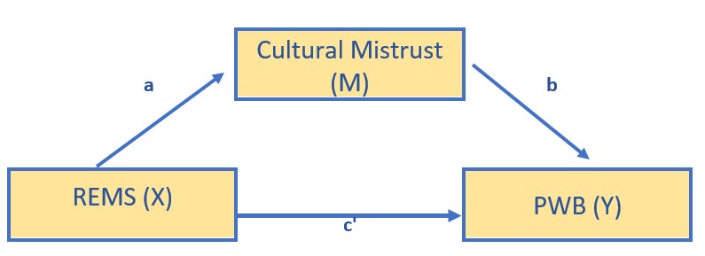
5.5.3 Specify the Model in lavaan
I am a big fan of “copying the model.” That is, I find code that works as a starting point. In specifying my model I used the simple mediation template from above. I
- replaced the Y, X, and M with variables names
- replacing the name of the df
- updated the object names (so I could use them in the same .rmd file)
modKim <- "
PWB ~ b*CMI + c_p*REMS
CMI ~a*REMS
indirect := a*b
direct := c_p
total_c := c_p + (a*b)
"set.seed(230916) #necessary for reproducible results since lavaan introduces randomness in the estimation proces
Kim_fit <- lavaan::sem(modKim, data = dfModel, se = "bootstrap", missing = "fiml")Kim_summary <- summary(Kim_fit, standardized = T, rsq = T, fit = TRUE,
ci = TRUE)
Kim_ParamEsts <- parameterEstimates(Kim_fit, boot.ci.type = "bca.simple",
standardized = TRUE)
Kim_summary## lavaan 0.6.17 ended normally after 1 iteration
##
## Estimator ML
## Optimization method NLMINB
## Number of model parameters 7
##
## Number of observations 156
## Number of missing patterns 1
##
## Model Test User Model:
##
## Test statistic 0.000
## Degrees of freedom 0
##
## Model Test Baseline Model:
##
## Test statistic 119.320
## Degrees of freedom 3
## P-value 0.000
##
## User Model versus Baseline Model:
##
## Comparative Fit Index (CFI) 1.000
## Tucker-Lewis Index (TLI) 1.000
##
## Robust Comparative Fit Index (CFI) 1.000
## Robust Tucker-Lewis Index (TLI) 1.000
##
## Loglikelihood and Information Criteria:
##
## Loglikelihood user model (H0) -218.515
## Loglikelihood unrestricted model (H1) -218.515
##
## Akaike (AIC) 451.030
## Bayesian (BIC) 472.379
## Sample-size adjusted Bayesian (SABIC) 450.222
##
## Root Mean Square Error of Approximation:
##
## RMSEA 0.000
## 90 Percent confidence interval - lower 0.000
## 90 Percent confidence interval - upper 0.000
## P-value H_0: RMSEA <= 0.050 NA
## P-value H_0: RMSEA >= 0.080 NA
##
## Robust RMSEA 0.000
## 90 Percent confidence interval - lower 0.000
## 90 Percent confidence interval - upper 0.000
## P-value H_0: Robust RMSEA <= 0.050 NA
## P-value H_0: Robust RMSEA >= 0.080 NA
##
## Standardized Root Mean Square Residual:
##
## SRMR 0.000
##
## Parameter Estimates:
##
## Standard errors Bootstrap
## Number of requested bootstrap draws 1000
## Number of successful bootstrap draws 1000
##
## Regressions:
## Estimate Std.Err z-value P(>|z|) ci.lower ci.upper
## PWB ~
## CMI (b) -0.189 0.052 -3.640 0.000 -0.291 -0.088
## REMS (c_p) -0.453 0.139 -3.260 0.001 -0.740 -0.194
## CMI ~
## REMS (a) 1.576 0.177 8.920 0.000 1.199 1.938
## Std.lv Std.all
##
## -0.189 -0.323
## -0.453 -0.286
##
## 1.576 0.584
##
## Intercepts:
## Estimate Std.Err z-value P(>|z|) ci.lower ci.upper
## .PWB 4.066 0.177 22.934 0.000 3.733 4.416
## .CMI 3.141 0.104 30.276 0.000 2.933 3.364
## Std.lv Std.all
## 4.066 9.004
## 3.141 4.072
##
## Variances:
## Estimate Std.Err z-value P(>|z|) ci.lower ci.upper
## .PWB 0.144 0.017 8.248 0.000 0.109 0.176
## .CMI 0.392 0.041 9.557 0.000 0.312 0.473
## Std.lv Std.all
## 0.144 0.706
## 0.392 0.659
##
## R-Square:
## Estimate
## PWB 0.294
## CMI 0.341
##
## Defined Parameters:
## Estimate Std.Err z-value P(>|z|) ci.lower ci.upper
## indirect -0.298 0.092 -3.251 0.001 -0.488 -0.138
## direct -0.453 0.139 -3.259 0.001 -0.740 -0.194
## total_c -0.750 0.112 -6.703 0.000 -0.961 -0.524
## Std.lv Std.all
## -0.298 -0.188
## -0.453 -0.286
## -0.750 -0.475## lhs op rhs label est se z pvalue ci.lower ci.upper
## 1 PWB ~ CMI b -0.189 0.052 -3.640 0.000 -0.284 -0.081
## 2 PWB ~ REMS c_p -0.453 0.139 -3.260 0.001 -0.754 -0.207
## 3 CMI ~ REMS a 1.576 0.177 8.920 0.000 1.196 1.937
## 4 PWB ~~ PWB 0.144 0.017 8.248 0.000 0.115 0.190
## 5 CMI ~~ CMI 0.392 0.041 9.557 0.000 0.320 0.487
## 6 REMS ~~ REMS 0.082 0.000 NA NA 0.082 0.082
## 7 PWB ~1 4.066 0.177 22.934 0.000 3.722 4.389
## 8 CMI ~1 3.141 0.104 30.276 0.000 2.941 3.367
## 9 REMS ~1 0.507 0.000 NA NA 0.507 0.507
## 10 indirect := a*b indirect -0.298 0.092 -3.251 0.001 -0.485 -0.131
## 11 direct := c_p direct -0.453 0.139 -3.259 0.001 -0.754 -0.207
## 12 total_c := c_p+(a*b) total_c -0.750 0.112 -6.703 0.000 -0.951 -0.518
## std.lv std.all std.nox
## 1 -0.189 -0.323 -0.323
## 2 -0.453 -0.286 -1.002
## 3 1.576 0.584 2.043
## 4 0.144 0.706 0.706
## 5 0.392 0.659 0.659
## 6 0.082 1.000 0.082
## 7 4.066 9.004 9.004
## 8 3.141 4.072 4.072
## 9 0.507 1.775 0.507
## 10 -0.298 -0.188 -0.659
## 11 -0.453 -0.286 -1.002
## 12 -0.750 -0.475 -1.6625.5.4 Interpret the Output
- Overall, our model accounted for 29% of the variance in the independent variable, well-being, and 34% of the variance in the mediator, cultural mistrust.
- a path: \(B = 1.576, p < 0.001\)
- b path: \(B = -0.189, p < 0.001\)
- the indirect effect is a product of the a and b paths: \(B = -0.298, p = 0.001\).
- The bias-corrected bootstrapped confidence intervals can sometimes be more lenient than \(p\) values; it is important they don’t cross zero \((95CI -0.485, -0.131 )\). If 0.00 is included in the confidence interval, then we cannot be confident that the estimate is not, itself, zero.
- the direct effect (c’, c prime, or c_p) is the isolated effect of X on Y when including M. We hope this value is lower than the total effect because it would mean that including M shared some of the variance in predicting Y. In our case the value for c’ is: \(B = -0.453, p = 0.001\). Unfortunately, they are significant and they are not markedly different from the total effect \((B = -0.750, p < 0.001)\).
- As a reminder, the total effect is is
- identical to the value of simply predicting Y on X (with no M it the model)
- the value of a(b) + c_p: \((1.576*-0.189) + (-0.453) = -0.750; p < 0.001)\)
5.5.5 A Figure and a Table
I make it a practice to immediately plot what I did. Because the plotting packages use our models, this can be a helpful self-check of our work.
# only worked when I used the library to turn on all these pkgs
library(lavaan)
library(dplyr)
library(ggplot2)
library(tidySEM)
tidySEM::graph_sem(model = Kim_fit) Hayes has great examples of APA style tables that have become the standard way to communicate results. I haven’t yet found a package that will turn this output into a journal-ready table, however with a little tinkering, we can approximate one of the standard tables. This code lets us understand the label names and how they are mapped
##      [,1]  [,2]
## [1,] NA    "REMS"
## [2,] "PWB" "CMI"
## attr(,"class")
## [1] "layout_matrix" "matrix"        "array"
We can write code to remap them
##      [,1]   [,2]  [,3]
## [1,] ""     "CMI" ""
## [2,] "REMS" ""    "PWB"
## attr(,"class")
## [1] "layout_matrix" "matrix"        "array"
We run again with our map and BOOM! Still needs tinkering for gorgeous, but hey!
tidySEM::graph_sem(Kim_fit, layout = med_map2, rect_width = 1.5, rect_height = 1.25,
    spacing_x = 2, spacing_y = 3, text_size = 4.5)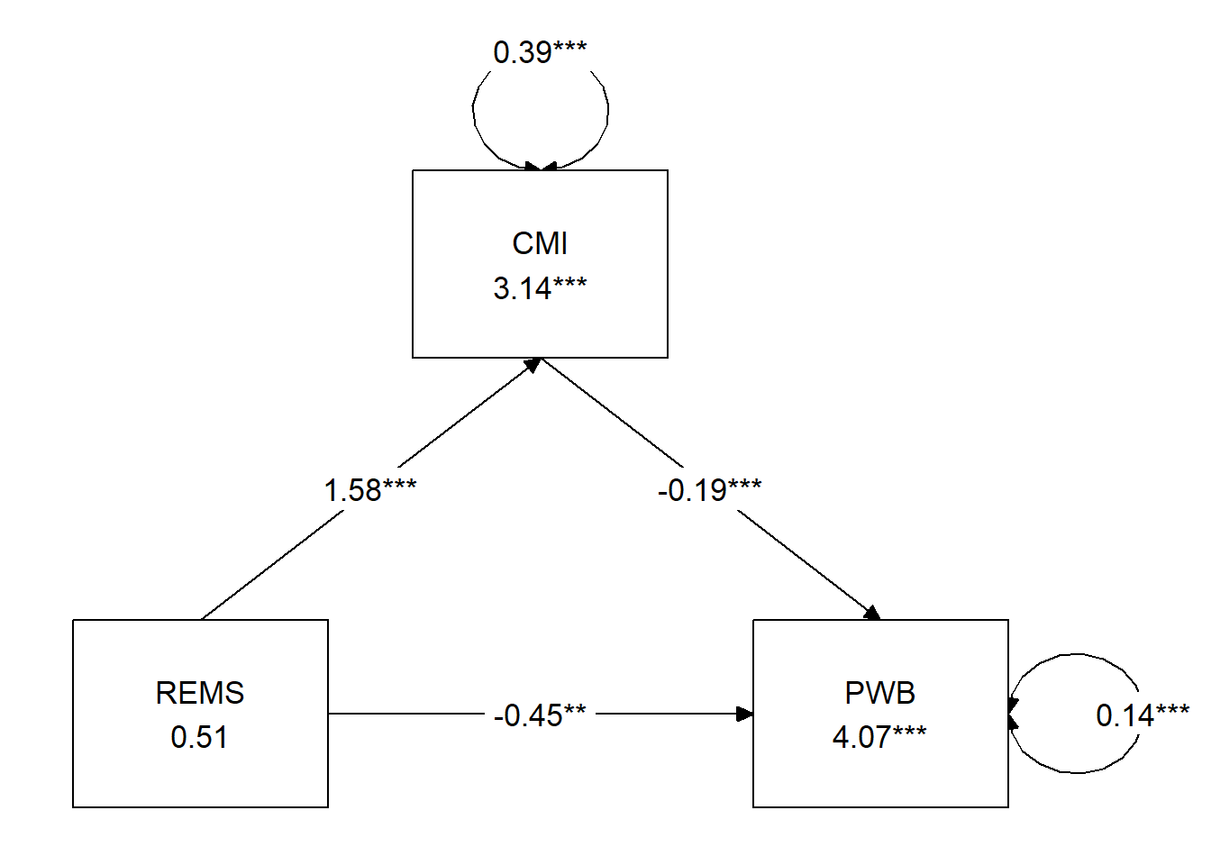
We can use simple code from base R to write the results to a .csv file. This makes it easier to create a table for presenting the results.
Here’s how I might organize the data.
Table 2
| Model Coefficients Assessing Cultural Mistrust as a Mediator Between Racial Microaggressions and Well-Being |
|---|
| Cultural Mistrust (M) | Well-Being (Y) |
| Antecedent | path | \(B\) | \(SE\) | \(p\) | path | \(B\) | \(SE\) | \(p\) |
| constant | \(i_{M}\) | 3.1419 | 0.103 | < 0.001 | \(i_{Y}\) | 4.066 | 0.177 | < 0.001 |
| REMS (X) | \(a\) | 1.576 | 0.184 | < 0.001 | \(c'\) | -0.453 | 0.139 | 0.001 |
| CMI (M) | \(b\) | -0.189 | 0.052 | < 0.001 |
| \(R^2\) = 34% | \(R^2\) = 29% |
| Note. The value of the indirect effect was \(B = -.298, SE = 0.092, p = 0.001, 95CI(-0.485,-0.131)\). |
5.5.6 Results
A simple mediation model examined the degree to which cultural mistrust mediated the relation of racial microaggressions on well-being. Using the lavaan package (v 0.6-16) in R, coefficients for each path, the indirect effect, and total effects were calculated. These values are presented in Table 2 and illustrated in Figure 2. Results suggested that racial/ethnic microaggressions had statistically significant effects on both cultural mistrust \((B = 1.576, p < 0.001)\) and well-being \((B = -0.453, p = 0.001)\). Further, the indirect effect from our simulated data was statistically significant (\(B = -.298, SE = 0.092, p = 0.001, 95CI[-0.485,-0.131])\). Results suggested that 34% of the variance in cultural mistrust and 29% of the variance in well-being were accounted for by the model.
5.6 Considering Covariates
Hayes Chapter 4 (2018) considers the role of covariates (e.g., other variables that could account for some of the variance in the model). When previous research (or commonsense, or detractors) suggest you should include them it is advisable to do so. If they are non-significant and/or your variables continue to explain variance over-and-above their contribution, then you have gained ground in ruling out plausible rival hypotheses and are adding to causal evidence.
Covariates are relatively easy to specify in lavaan. I tend to look at my figure and “see where the arrows go.” Those translate readily to the equations we write in the lavaan code.
Let’s say we are concerned that anxiety covaries with cultural mistrust and well-being We’ll add it as a covariate to both.
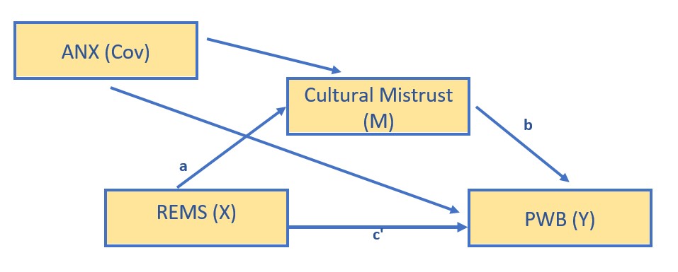
Kim_fit_covs <- "
          PWB ~ b*CMI + c_p*REMS
          CMI ~a*REMS
          CMI ~ covM*ANX
          PWB ~ covY*ANX

          indirect :=  a*b
          direct  := c_p
          total_c  := c_p + (a*b)

          "
set.seed(230916)  #needed for reproducibility especially when specifying bootstrapped confidence intervals
Kim_fit_covs <- lavaan::sem(Kim_fit_covs, data = dfKim, se = "bootstrap",
    missing = "fiml")
Kcov_sum <- lavaan::summary(Kim_fit_covs, standardized = T, rsq = T, fit = TRUE,
    ci = TRUE)
Kcov_ParEsts <- lavaan::parameterEstimates(Kim_fit_covs, boot.ci.type = "bca.simple",
    standardized = TRUE)
Kcov_sum
## lavaan 0.6.17 ended normally after 1 iteration
##
## Estimator ML
## Optimization method NLMINB
## Number of model parameters 9
##
## Number of observations 156
## Number of missing patterns 1
##
## Model Test User Model:
##
## Test statistic 0.000
## Degrees of freedom 0
##
## Model Test Baseline Model:
##
## Test statistic 136.009
## Degrees of freedom 5
## P-value 0.000
##
## User Model versus Baseline Model:
##
## Comparative Fit Index (CFI) 1.000
## Tucker-Lewis Index (TLI) 1.000
##
## Robust Comparative Fit Index (CFI) 1.000
## Robust Tucker-Lewis Index (TLI) 1.000
##
## Loglikelihood and Information Criteria:
##
## Loglikelihood user model (H0) -210.170
## Loglikelihood unrestricted model (H1) -210.170
##
## Akaike (AIC) 438.341
## Bayesian (BIC) 465.789
## Sample-size adjusted Bayesian (SABIC) 437.301
##
## Root Mean Square Error of Approximation:
##
## RMSEA 0.000
## 90 Percent confidence interval - lower 0.000
## 90 Percent confidence interval - upper 0.000
## P-value H_0: RMSEA <= 0.050 NA
## P-value H_0: RMSEA >= 0.080 NA
##
## Robust RMSEA 0.000
## 90 Percent confidence interval - lower 0.000
## 90 Percent confidence interval - upper 0.000
## P-value H_0: Robust RMSEA <= 0.050 NA
## P-value H_0: Robust RMSEA >= 0.080 NA
##
## Standardized Root Mean Square Residual:
##
## SRMR 0.000
##
## Parameter Estimates:
##
## Standard errors Bootstrap
## Number of requested bootstrap draws 1000
## Number of successful bootstrap draws 1000
##
## Regressions:
## Estimate Std.Err z-value P(>|z|) ci.lower ci.upper
## PWB ~
## CMI (b) -0.163 0.051 -3.212 0.001 -0.263 -0.068
## REMS (c_p) -0.219 0.149 -1.474 0.140 -0.519 0.071
## CMI ~
## REMS (a) 1.349 0.191 7.045 0.000 0.956 1.707
## ANX (covM) 0.198 0.096 2.067 0.039 0.009 0.379
## PWB ~
## ANX (covY) -0.238 0.061 -3.910 0.000 -0.349 -0.109
## Std.lv Std.all
##
## -0.163 -0.279
## -0.219 -0.139
##
## 1.349 0.500
## 0.198 0.145
##
## -0.238 -0.299
##
## Intercepts:
## Estimate Std.Err z-value P(>|z|) ci.lower ci.upper
## .PWB 4.521 0.209 21.595 0.000 4.111 4.936
## .CMI 2.697 0.245 11.004 0.000 2.236 3.182
## Std.lv Std.all
## 4.521 10.011
## 2.697 3.497
##
## Variances:
## Estimate Std.Err z-value P(>|z|) ci.lower ci.upper
## .PWB 0.132 0.016 8.210 0.000 0.098 0.161
## .CMI 0.384 0.040 9.708 0.000 0.304 0.461
## Std.lv Std.all
## 0.132 0.648
## 0.384 0.645
##
## R-Square:
## Estimate
## PWB 0.352
## CMI 0.355
##
## Defined Parameters:
## Estimate Std.Err z-value P(>|z|) ci.lower ci.upper
## indirect -0.220 0.076 -2.888 0.004 -0.377 -0.082
## direct -0.219 0.149 -1.473 0.141 -0.519 0.071
## total_c -0.440 0.122 -3.612 0.000 -0.675 -0.209
## Std.lv Std.all
## -0.220 -0.139
## -0.219 -0.139
## -0.440 -0.278## lhs op rhs label est se z pvalue ci.lower ci.upper
## 1 PWB ~ CMI b -0.163 0.051 -3.212 0.001 -0.257 -0.056
## 2 PWB ~ REMS c_p -0.219 0.149 -1.474 0.140 -0.528 0.062
## 3 CMI ~ REMS a 1.349 0.191 7.045 0.000 0.910 1.673
## 4 CMI ~ ANX covM 0.198 0.096 2.067 0.039 0.009 0.377
## 5 PWB ~ ANX covY -0.238 0.061 -3.910 0.000 -0.353 -0.110
## 6 PWB ~~ PWB 0.132 0.016 8.210 0.000 0.107 0.169
## 7 CMI ~~ CMI 0.384 0.040 9.708 0.000 0.320 0.479
## 8 REMS ~~ REMS 0.082 0.000 NA NA 0.082 0.082
## 9 REMS ~~ ANX 0.094 0.000 NA NA 0.094 0.094
## 10 ANX ~~ ANX 0.320 0.000 NA NA 0.320 0.320
## 11 PWB ~1 4.521 0.209 21.595 0.000 4.114 4.941
## 12 CMI ~1 2.697 0.245 11.004 0.000 2.232 3.180
## 13 REMS ~1 0.507 0.000 NA NA 0.507 0.507
## 14 ANX ~1 2.824 0.000 NA NA 2.824 2.824
## 15 indirect := a*b indirect -0.220 0.076 -2.888 0.004 -0.385 -0.085
## 16 direct := c_p direct -0.219 0.149 -1.473 0.141 -0.528 0.062
## 17 total_c := c_p+(a*b) total_c -0.440 0.122 -3.612 0.000 -0.673 -0.206
## std.lv std.all std.nox
## 1 -0.163 -0.279 -0.279
## 2 -0.219 -0.139 -0.485
## 3 1.349 0.500 1.749
## 4 0.198 0.145 0.256
## 5 -0.238 -0.299 -0.528
## 6 0.132 0.648 0.648
## 7 0.384 0.645 0.645
## 8 0.082 1.000 0.082
## 9 0.094 0.580 0.094
## 10 0.320 1.000 0.320
## 11 4.521 10.011 10.011
## 12 2.697 3.497 3.497
## 13 0.507 1.775 0.507
## 14 2.824 4.995 2.824
## 15 -0.220 -0.139 -0.488
## 16 -0.219 -0.139 -0.485
## 17 -0.440 -0.278 -0.9745.6.1 A Figure and a Table
Let’s look at a figure to see see if we did what we think we did. And to also get a graphic representation of our results.
# only worked when I used the library to turn on all these pkgs
library(lavaan)
library(dplyr)
library(ggplot2)
library(tidySEM)
tidySEM::graph_sem(model = Kim_fit_covs)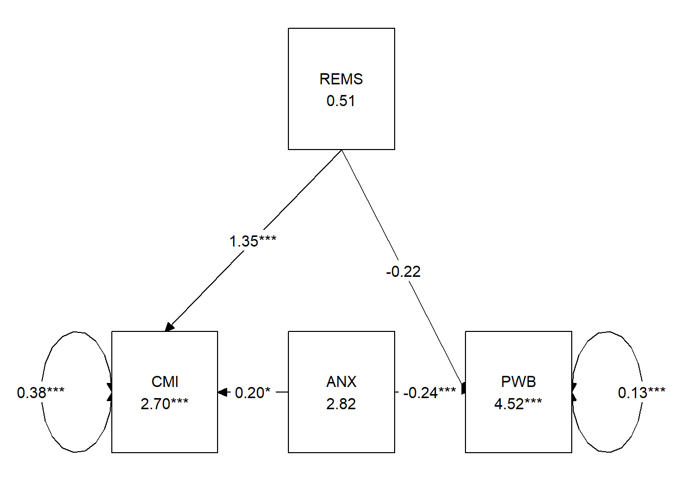
##      [,1]  [,2]   [,3]
## [1,] NA    "REMS" NA
## [2,] "CMI" "ANX"  "PWB"
## attr(,"class")
## [1] "layout_matrix" "matrix"        "array"
We can write code to remap them
##      [,1]   [,2] [,3]  [,4]
## [1,] "ANX"  ""   "CMI" ""
## [2,] "REMS" ""   ""    "PWB"
## attr(,"class")
## [1] "layout_matrix" "matrix"        "array"
We run again with our map and BOOM! Still needs tinkering for gorgeous, but hey!
tidySEM::graph_sem(Kim_fit_covs, layout = med_map3, rect_width = 1.5, rect_height = 1.25,
    spacing_x = 2, spacing_y = 3, text_size = 4.5)
Below is code to create an outfile that could help with creating a table in a word document or spreadsheet. There will be output that is produced with SEM models that won’t be relevant for this project.
Table 3
| Model Coefficients Assessing Cultural Mistrust as a Mediator Between Racial Microaggressions and Well-Being |
|---|
| Cultural Mistrust (M) | Well-Being (Y) |
| Antecedent | path | \(B\) | \(SE\) | \(p\) | path | \(B\) | \(SE\) | \(p\) |
| constant | \(i_{M}\) | 2.697 | 0.245 | <0.001 | \(i_{Y}\) | 4.521 | 0.209 | <0.001 |
| REMS (X) | \(a\) | 1.349 | 0.191 | <0.001 | \(c'\) | -0.219 | 0.149 | 0.140 |
| CMI (M) | \(b\) | -0.163 | 0.051 | 0.001 | ||||
| ANX (Cov) | 0.198 | 0.096 | 0.039 | -0.238 | 0.061 | <0.001 |
| \(R^2\) = 36% | \(R^2\) = 35% |
| Note. The value of the indirect effect was \(B = -.220, SE = 0.076, p = 0.004, 95CI(-0.385,-0.085)\). |
5.6.2 APA Style Write-up
There are varying models for reporting the results of mediation. The Kim et al. (Paul Youngbin Kim et al., 2017) writeup is a great example. Rather than copying it directly, I have modeled my table after the ones in Hayes (2018) text. You’ll notice that information in the table and text are minimally overlapping. APA style cautions us against redundancy in text and table.
Results
A simple mediation model examined the degree to which cultural mistrust mediated the effect of racial microaggressions on psychological well-being. Using the lavaan package (v 0.6-16) in R, coefficients for the each path, the indirect effect, and total effects were calculated. Additionally, the effect of covariate, anxiety, was mapped onto both the mediator and dependent variable. The model accounted for 36% of the variance in cultural mistrust and 35% of the variance in well-being. Supporting the notion of a mediated model, there was a statistically significant indirect effect \((B = -.220, SE = 0.076, p = 0.004, 95CI[-0.385,-0.085])\) in combination with a non-significant direct effect \((B = -0.219, p = 0.140)\) and a statistically significant total effect\((B = -0.440, p < 0.001)\).
5.7 STAY TUNED
A section on power analysis is planned and coming soon! My apologies that it’s not quite Ready.
5.9 Practice Problems
The three problems described below are designed to grow with the subsequent chapters on complex mediation and conditional process analysis (i.e,. moderated mediation). Therefore, I recommend that you select a dataset that includes at least four variables. If you are new to this topic, you may wish to select variables that are all continuously scaled. The IV and moderator (subsequent chapters) could be categorical (if they are dichotomous, please use 0/1 coding; if they have more than one category it is best if they are ordered). You will likely encounter challenges that were not covered in this chapter. Search for and try out solutions, knowing that there are multiple paths through the analysis.
The suggested practice problem for this chapter is to conduct a simple mediation.
5.9.1 Problem #1: Rework the research vignette as demonstrated, but change the random seed
If this topic feels a bit overwhelming, simply change the random seed in the data simulation, then rework the problem. This should provide minor changes to the data (maybe in the second or third decimal point), but the results will likely be very similar.
5.9.2 Problem #2: Rework the research vignette, but swap one or more variables
Use the simulated data, but select one of the other models that was evaluated in the Kim et al. (2017) study. Compare your results to those reported in the mansucript.
5.9.3 Problem #3: Use other data that is available to you
Using data for which you have permission and access (e.g., IRB approved data you have collected or from your lab; data you simulate from a published article; data from an open science repository; data from other chapters in this OER), complete a simple mediation.
5.9.4 Grading Rubric
| Assignment Component | Points Possible | Points Earned |
|---|---|---|
| 1. Assign each variable to the X, Y, or M roles (ok but not required to include a cov) | 5 | _____ |
| 2. Import the data and format the variables in the model | 5 | _____ |
| 3. Specify and run the lavaan model | 5 | _____ |
| 4. Use tidySEM to create a figure that represents your results | 5 | _____ |
| 5. Create a table that includes regression output for the M and Y variables | 5 | _____ |
| 6. Represent your work in an APA-style write-up | 5 | _____ |
| 7. Explanation to grader | 5 | _____ |
| 8. Be able to hand-calculate the indirect, direct, and total effects from the a, b, & c’ paths | 5 | _____ |
| Totals | 35 | _____ |
5.10 Homeworked Example
For more information about the data used in this homeworked example, please refer to the description and codebook located at the end of the introductory lesson in ReCentering Psych Stats. An .rds file which holds the data is located in the Worked Examples folder at the GitHub site the hosts the OER. The file name is ReC.rds.
The suggested practice problem for this chapter is to conduct a simple mediation.
5.10.1 Assign each variable to the X, Y, or M roles (ok but not required to include a covariate)
X = Centering: explicit recentering (0 = precentered; 1 = recentered) M = TradPed: traditional pedagogy (continuously scaled with higher scores being more favorable) Y = SRPed: socially responsive pedagogy (continuously scaled with higher scores being more favorable)
Specify a research model
I am hypothesizing that the evaluation of social responsive pedagogy is predicted by intentional recentering through traditional pedagogy.
Import the data and format the variables in the model
I need to score the TradPed and SRPed variables
TradPed_vars <- c("ClearResponsibilities", "EffectiveAnswers", "Feedback",
    "ClearOrganization", "ClearPresentation")
raw$TradPed <- sjstats::mean_n(raw[, ..TradPed_vars], 0.75)

SRPed_vars <- c("InclusvClassrm", "EquitableEval", "MultPerspectives",
    "DEIintegration")
raw$SRPed <- sjstats::mean_n(raw[, ..SRPed_vars], 0.75)
I will create a babydf.
Let’s check the structure of the variables:
str(babydf)Specify and run the lavaan model
ReCMed <- "
          SRPed ~ b*TradPed + c_p*Centering
          TradPed ~ a*Centering

          indirect :=  a*b
          direct  := c_p
          total_c  := c_p + (a*b)
          "

set.seed(231002)  #needed for reproducible results since lavaan introduced randomness into some procedures
ReCfit <- lavaan::sem(ReCMed, data = babydf, se = "bootstrap", missing = "fiml")
ReCsummary <- lavaan::summary(ReCfit, standardized = T, rsq = T, fit = TRUE,
    ci = TRUE)
ReC_ParamEsts <- lavaan::parameterEstimates(ReCfit, boot.ci.type = "bca.simple",
    standardized = TRUE)
ReCsummary
## lavaan 0.6.17 ended normally after 14 iterations
##
## Estimator ML
## Optimization method NLMINB
## Number of model parameters 7
##
## Number of observations 310
## Number of missing patterns 4
##
## Model Test User Model:
##
## Test statistic 0.000
## Degrees of freedom 0
##
## Model Test Baseline Model:
##
## Test statistic 216.492
## Degrees of freedom 3
## P-value 0.000
##
## User Model versus Baseline Model:
##
## Comparative Fit Index (CFI) 1.000
## Tucker-Lewis Index (TLI) 1.000
##
## Robust Comparative Fit Index (CFI) 1.000
## Robust Tucker-Lewis Index (TLI) 1.000
##
## Loglikelihood and Information Criteria:
##
## Loglikelihood user model (H0) -506.434
## Loglikelihood unrestricted model (H1) -506.434
##
## Akaike (AIC) 1026.868
## Bayesian (BIC) 1053.024
## Sample-size adjusted Bayesian (SABIC) 1030.823
##
## Root Mean Square Error of Approximation:
##
## RMSEA 0.000
## 90 Percent confidence interval - lower 0.000
## 90 Percent confidence interval - upper 0.000
## P-value H_0: RMSEA <= 0.050 NA
## P-value H_0: RMSEA >= 0.080 NA
##
## Robust RMSEA 0.000
## 90 Percent confidence interval - lower 0.000
## 90 Percent confidence interval - upper 0.000
## P-value H_0: Robust RMSEA <= 0.050 NA
## P-value H_0: Robust RMSEA >= 0.080 NA
##
## Standardized Root Mean Square Residual:
##
## SRMR 0.000
##
## Parameter Estimates:
##
## Standard errors Bootstrap
## Number of requested bootstrap draws 1000
## Number of successful bootstrap draws 1000
##
## Regressions:
## Estimate Std.Err z-value P(>|z|) ci.lower ci.upper
## SRPed ~
## TradPed (b) 0.549 0.046 12.067 0.000 0.458 0.645
## Centerng (c_p) 0.127 0.047 2.684 0.007 0.036 0.219
## TradPed ~
## Centerng (a) -0.101 0.090 -1.121 0.262 -0.287 0.080
## Std.lv Std.all
##
## 0.549 0.716
## 0.127 0.107
##
## -0.101 -0.066
##
## Intercepts:
## Estimate Std.Err z-value P(>|z|) ci.lower ci.upper
## .SRPed 2.006 0.231 8.689 0.000 1.543 2.442
## .TradPed 4.394 0.139 31.707 0.000 4.109 4.675
## Std.lv Std.all
## 2.006 3.440
## 4.394 5.778
##
## Variances:
## Estimate Std.Err z-value P(>|z|) ci.lower ci.upper
## .SRPed 0.165 0.017 9.467 0.000 0.130 0.203
## .TradPed 0.576 0.070 8.225 0.000 0.444 0.724
## Std.lv Std.all
## 0.165 0.486
## 0.576 0.996
##
## R-Square:
## Estimate
## SRPed 0.514
## TradPed 0.004
##
## Defined Parameters:
## Estimate Std.Err z-value P(>|z|) ci.lower ci.upper
## indirect -0.056 0.052 -1.077 0.282 -0.168 0.042
## direct 0.127 0.047 2.682 0.007 0.036 0.219
## total_c 0.071 0.068 1.045 0.296 -0.055 0.204
## Std.lv Std.all
## -0.056 -0.047
## 0.127 0.107
## 0.071 0.060## lhs op rhs label est se z pvalue ci.lower ci.upper
## 1 SRPed ~ TradPed b 0.549 0.046 12.067 0.000 0.459 0.645
## 2 SRPed ~ Centering c_p 0.127 0.047 2.684 0.007 0.032 0.211
## 3 TradPed ~ Centering a -0.101 0.090 -1.121 0.262 -0.292 0.075
## 4 SRPed ~~ SRPed 0.165 0.017 9.467 0.000 0.135 0.209
## 5 TradPed ~~ TradPed 0.576 0.070 8.225 0.000 0.462 0.741
## 6 Centering ~~ Centering 0.241 0.000 NA NA 0.241 0.241
## 7 SRPed ~1 2.006 0.231 8.689 0.000 1.534 2.433
## 8 TradPed ~1 4.394 0.139 31.707 0.000 4.114 4.683
## 9 Centering ~1 1.406 0.000 NA NA 1.406 1.406
## 10 indirect := a*b indirect -0.056 0.052 -1.077 0.282 -0.171 0.038
## 11 direct := c_p direct 0.127 0.047 2.682 0.007 0.032 0.211
## 12 total_c := c_p+(a*b) total_c 0.071 0.068 1.045 0.296 -0.053 0.205
## std.lv std.all std.nox
## 1 0.549 0.716 0.716
## 2 0.127 0.107 0.217
## 3 -0.101 -0.066 -0.133
## 4 0.165 0.486 0.486
## 5 0.576 0.996 0.996
## 6 0.241 1.000 0.241
## 7 2.006 3.440 3.440
## 8 4.394 5.778 5.778
## 9 1.406 2.863 1.406
## 10 -0.056 -0.047 -0.096
## 11 0.127 0.107 0.217
## 12 0.071 0.060 0.122Use tidySEM to create a figure that represents your results
# only worked when I used the library to turn on all these pkgs
library(lavaan)
library(dplyr)
library(ggplot2)
library(tidySEM)
tidySEM::graph_sem(model = ReCfit)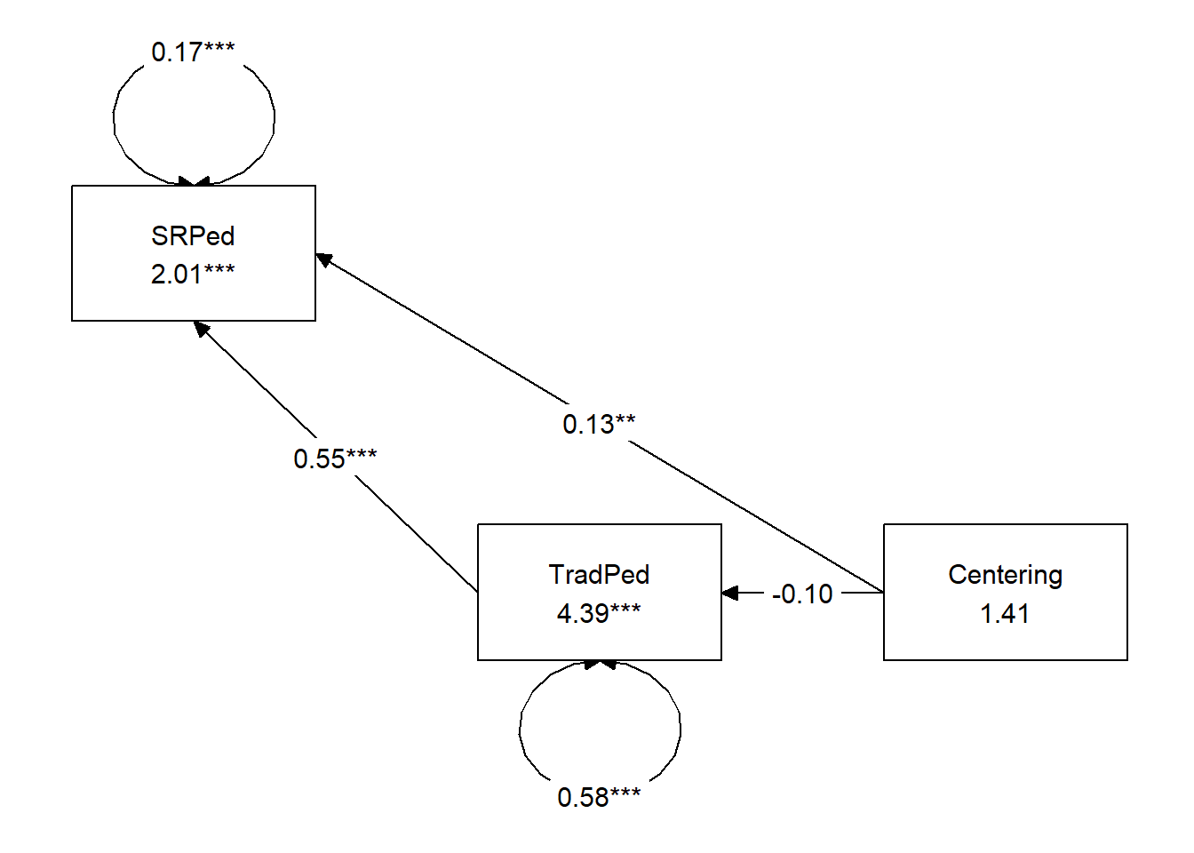
##      [,1]    [,2]      [,3]
## [1,] "SRPed" "TradPed" "Centering"
## attr(,"class")
## [1] "layout_matrix" "matrix"        "array"
We can write code to remap them
##      [,1]        [,2]      [,3]
## [1,] ""          "TradPed" ""
## [2,] "Centering" ""        "SRPed"
## attr(,"class")
## [1] "layout_matrix" "matrix" "array"tidySEM::graph_sem(ReCfit, layout=med_map, rect_width = 1.5, rect_height = 1.25, spacing_x = 2, spacing_y = 3, text_size = 4.5)
Create a table that includes regression output for the M and Y variables
Table 1
| Model Coefficients Assessing Traditional Pedagogy as a Mediator Between Centering and Socially Responsive Pedagogy |
|---|
| Traditional Pedagogy (M) | Socially Responsive Pedagogy (Y) |
| Antecedent | path | \(B\) | \(SE\) | \(p\) | path | \(B\) | \(SE\) | \(p\) |
| constant | \(i_{M}\) | 4.394 | 0.139 | < 0.001 | \(i_{Y}\) | 2.006 | 0.231 | < 0.001 |
| Centering (X) | \(a\) | -0.101 | 0.090 | 0.262 | \(c'\) | 0.127 | 0.047 | 0.007 |
| TradPed (M) | \(b\) | 0.549 | 0.046 | < 0.001 |
| \(R^2\) = 0.4% | \(R^2\) = 51% |
| Note. Centering: 0 = pre-centered, 1 = recentered. TradPed is traditional pedagogy. The value of the indirect effect was \(B = -0.056, SE = 0.051, p = 0.272, 95CI(-0.163,0.035)\) |
Represent your work in an APA-style write-up
A simple mediation model examined the degree to which evaluations of traditional pedagogy mediated the relation of explicit recentering on socially responsive pedagogy. Using the lavaan package (v 0.6-16) in R, coefficients for each path, the indirect effect, and total effects were calculated. These values are presented in Table 1 and illustrated in Figure 1. Results suggested that neglibible (.4%) of the variance was accounted for in traditional pedagogy. In contrast 51% of the variance was accounted for in socially responsive pedagogy. The indirect effect \((B = -0.056, SE = 0.051, p = 0.272, 95CI[-0.163,0.035])\) was statistically significant. Comparing total and direct effects, the total effect of centering and traditional pedagogy on socially responsive pedagogy was not statistically significant \((B = 0.071, p = 0.302)\). In contrast, the direct effect was (\(B = 0.127, p = 0.008\) was not). This suggests that while centering and traditional pedagogy do influence socially responsive pedagogy, their influence is relatively independent.
apaTables::apa.cor.table(babydf, table.number = 1, show.sig.stars = TRUE,
    landscape = TRUE, filename = NA)
##
##
## Table 1
##
## Means, standard deviations, and correlations with confidence intervals
##
##
## Variable M SD 1
## 1. TradPed 4.25 0.76
##
## 2. SRPed 4.52 0.58 .71**
## [.65, .76]
##
##
## Note. M and SD are used to represent mean and standard deviation, respectively.
## Values in square brackets indicate the 95% confidence interval.
## The confidence interval is a plausible range of population correlations
## that could have caused the sample correlation (Cumming, 2014).
## * indicates p < .05. ** indicates p < .01.
##