Chapter 2 Scoring

Screencasted Lecture Link

The focus of this chapter is to continue the process of scrubbing-and-scoring. We continue with the raw data we downloaded and prepared in the prior chapter. In this chapter we analyze and manage missingness, score scales/subscales, and represent our work with an APA-style write-up. To that end, we will address the conceptual considerations and practical steps in this process.

2.1 Navigating this Lesson

There is about 1 hour and 20 minutes of lecture. If you work through the materials with me it would be good to add another hour.

While the majority of R objects and data you will need are created within the R script that sources the chapter, there are a few that cannot be created from within the R framework. Additionally, sometimes links fail. All original materials are provided at the Github site that hosts the book. More detailed guidelines for ways to access all these materials are provided in the OER’s introduction

2.1.1 Learning Objectives

Learning objectives from this lecture include the following:

Recognize the key components of data loss mechanisms (MCAR, MAR, MNAR), including how to diagnose MCAR.
Interpret missingness figures produced by packages such as mice.
Articulate a workflow for scrubbing and scoring data.
Use critical data manipulation functions from dplyr including filter(), select(), and mutate() to prepare variables.
Interpret code related to missingness (i.e., “is.na”, “!is.na”) and the pipe (%>%)

2.1.2 Planning for Practice

The suggestions for practice continue from the prior chapter. The assignment in the prior chapter involved downloading a dataset from Qualtrics and the “scrubbing” it on the basis of inclusion and exclusion criteria. Using that same data, the practice suggestions in this chapter will continue to use Parent’s (2013) AIA approach to managing missing data, to score the variables of interest. Options of graded complexity could incude:

Repeating the steps in the chapter with the most recent data from the Rate-A-Recent-Course survey; differences will be in the number of people who have completed the survey since the chapter was written.
Use the dataset that is the source of the chapter, but score a different set of items that you choose.
Begin with raw data to which you have access.

2.1.3 Readings & Resources

In preparing this chapter, I drew heavily from the following resource(s). Other resources are cited (when possible, linked) in the text with complete citations in the reference list.

Enders, C. K. (2010). Applied missing data analysis (2010-13190-000). Guilford Press.
- Enders’ text continues to be the comprehensive “go-to” source for examining and managing missing data.
Kline, R. B. (2016). Data preparation and psychometrics review. In Principles and Practice of Structural Equation Modeling, Fourth Edition. Guilford Publications. http://ebookcentral.proquest.com/lib/spu/detail.action?docID=4000663
- Kline’s chapter is my “go-to” for making decisions about preparing data for analysis.
Parent, M. C. (2013). Handling item-level missing data: Simpler is just as good. The Counseling Psychologist, 41(4), 568–600. https://doi.org/10.1177/0011000012445176
- The purpose of Parent’s article was to argue that complex and resource-intensive procedurs like multiple imputation are unnecessary. Following a simulation that supports his claims, Parent provides some guidelines to follow for the AIA approach.

2.1.4 Packages

The packages used in this lesson are embedded in this code. When the hashtags are removed, the script below will (a) check to see if the following packages are installed on your computer and, if not (b) install them.

# if(!require(tidyverse)){install.packages('tidyverse')}
# if(!require(psych)){install.packages('psych')}
# if(!require(mice)){install.packages('mice')}
# if(!require(sjstats)){install.packages('sjstats')}
# if(!require(formattable)){install.packages('formattable')}

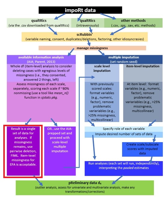
2.2 Workflow for Scoring

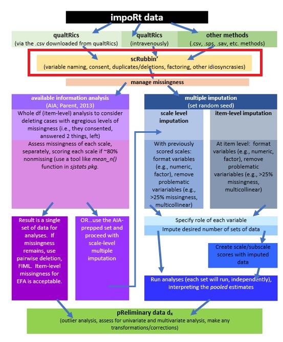
The following is a proposed workflow for preparing data for analysis.

The same workflow guides us through the Scrubbing, Scoring, and Data Dx chapters. At this stage in the chapter we are still scrubbing as we work through the item-level and whole-level portions of the AIA (left side) of the chart.

An image of our stage in the workflow for scrubbing and scoring data.

2.3 Research Vignette

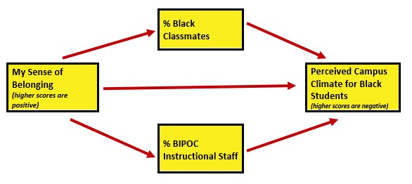
The research vignette comes from the survey titled, Rate-a-Recent-Course: A ReCentering Psych Stats Exercise and is explained in the prior chapter. In the prior chapter we conducted super-preliminary scrubbing of variables that will allow us to examine the respondent’s perceived campus climate for students who are Black, predicted by the the respondent’s own campus belonging, and also the structural diversity proportions of Black students in the classroom and the BIPOC instructional staff. At present, I see this as a parallel mediation. That is, the perceived campus climate for Black students will be predicted by the respondent’s sense of belonging, through the proportion of Black classmates and BIPOC (Black, Indigenous, and people of color)instructional staff.

I would like to assess the model by having the instructional staff variable to be the percent of Black instructional staff. At the time that this lecture is being prepared, there is insufficient representation of Black faculty to model this.

An image of the statistical model for which we are preparing data.

First, though, let’s take a more conceptual look at issues regarding missing data. We’ll come back to details of the survey as we work with it.

2.4 On Missing Data

On the topic of missing data, we follow the traditions in most textbooks. We start by considering data loss mechanisms and options for managing missingness.

Although the workflow I recommend is fairly straightforward, the topic is not. Quantitative psychologist have produced volumes of research that supports and refutes all of these issues in detail. An in-deth review of this is found in Enders’ (2010) text.

2.4.1 Data Loss Mechanisms

We generally classify missingess in data in three different ways (Kline, 2016b; Parent, 2013):

Missing completely at random (MCAR) is the ideal case (and often unrealistic in actual data). For variable Y this mean that

Missingness is due to a factor(s) completely unrelated to the missing data. Stated another way:
- Missing observations differ from the observed scores only by chance; that is, whether scores on Y are missing or not missing is unrelated to Y itself
The presence versus absence of data on Y is unrelated to all other variables in the dataset. That is, the nonmissing data are just a random sample of scores that the researcher would have analyzed had the data been complete. We might think of it as haphazard missing.
- A respondent is interrupted, looks up, looks down, and skips an item.
- A computer glitch causes spotty missingness – unrelated to any particular variable.

MCAR is the ideal state because results from it should not be biased as a function of the missingness.

Missing at random (MAR) missing data arise from a process that is both measured and predictable in a particular sample. Admittedly the use of “random” in this term is odd, because, by definition, the missingness is not random.

Restated:

Missingness on Y is unrelated to Y itself, but
Missingness is on Y is correlated with other variables in the data set.

Example: Men are less likely to respond to questions about mental health than women, but among men, the probability of responding is unrelated to their true mental health status.

Kline (2016b) indicated that information loss due to MAR is potentially recoverable through imputation where missing scores are replaced by predicted scores. The predicted scores are generated from other variables in the data set that predict missingness on Y. If the strength of that prediction is reasonably strong, then results on Y after imputation may be relatively unbiased. In this sense, the MAR pattern is described as ignorable with regard to potential bias. Two types of variables can be used to predict the missing data

variables that are in the prediction equation, and
auxiliary variables (i.e., variables in the dataset that are not in the prediction equation).

Parent (2013) noted that multiple imputation and expectation maximization have frequently been used to manage missingness in MAR circumstances.

Missing not at random (MNAR) is when the presence versus absence of scores on Y depend on Y itself. This is non-ignorable.

For example, if a patient drops out of a medical RCT because there are unpleasant side effects from the treatment, this discomfort is not measured, but the data is missing due to a process that is unknown in a particular data set. Results based on complete cases only can be severely biased when the data loss pattern is MNAR. That is, a treatment may look more beneficial than it really is if data from patients who were unable to tolerate the treatment are lost.

Parent (2013) described MNAR a little differently – but emphasized that the systematic missingness would be related to a variable outside the datset. Parent provided the example of items written in a manner that may be inappropriate for some participants (e.g., asking women about a relationship with their boyfriend/husband, when the woman might be in same gender relationship). If there were not demographic items that could identify the bias, this would be MNAR. Parent strongly advises researchers to carefully proofread and pilot surveys to avoid MNAR circumstances.

Kline (2016b) noted that the choice of the method to deal with the incomplete records can make a difference in the results, and should be made carefully.

2.4.2 Diagnosing Missing Data Mechanisms

The bad news is that we never really know (with certainty) the type of missing data mechanism in our data. The following tools can help understand the mechanisms that contribute to missingness.

Missing data analyses often includes correlations that could predict missingness.
Little and Rubin (2002) proposed a multivariate statistical test of the MCAR assumption that simultaneously compares complete versus incomplete cases on Y across all other variables. If this comparison is significant, then the MCAR hypothesis is rejected.
- To restate: we want a non-significant result; and we use the sometimes-backwards-sounding NHST (null hypothesis significance testing) language, “MCAR cannot be rejected.”
MCAR can also be examined through a series of t tests of the cases that have missing scores on Y with cases that have complete records on other variables. Unfortunately, sample sizes contribute to problems with interpretation. With low samples, they are underpowered; in large samples they can flag trivial differences.

If MCAR is rejected, we are never sure whether the data loss mechanism is MAR or MNAR. There is no magical statistical “fix.” Kline (2016b) wrote, “About the best that can be done is to understand the nature of the underlying data loss pattern and accordingly modify your interpretation of the results” (p. 85).

2.4.3 Managing Missing Data

There are a number of approaches to managing missing data. Here is a summary of the ones most commonly used.

Listwise deletion (aka, Complete Case Analysis) If there is a missing score on any variable, that case is excluded from all analyses.
Pairwise deletion Cases are excluded only if they have missing data on variables involved in a particular analysis. AIA is a variant of pair-wise deletion, but it preserves as much data as possible with person-mean imputation at the scale level.
Mean/median substitution Mean/median substitution replaces missing values with the mean/median of that particular variable. While this preserves the mean of the dataset, it can cause bias by decreasing variance. For example, if you have a column that has substantial of missingness and you replace each value with the same, fixed, mean, the variability of that variable has just been reduced. A variation on this is a group-mean substitution where the missing score in a particular group (e.g., women) is replaced by the group mean.
Full information maximum likelihood (FIML) A model-based method that takes the researcher’s model as the starting point. The procedure partitions the cases in a raw data file into subsets, each with the same pattern of missing observations, including none (complete cases). Statistical information (e.g., means, variances) is extracted from each subset so all case are retained in the analysis. Parameters for the researcher’s model are estimated after combining all available information over the subsets of cases.
Multiple imputation A data based method that works with the whole raw data file (not just with the observed variables that comprise the researcher’s model). Multiple imputation assumes that data are MAR (remember, MCAR is the more prestigious one). This means that researchers assume that missing values can be replaced by predictions derived from the observable portion fo the dataset.
- Multiple datasets (often 5 to 20) are created where missing values are replaced via a randomized process (so the same missing value [item 4 for person A] will likely have different values for each dataset).
- The desired anlayis(es) is conducted simultaneously/separately for each of the imputed sets (so if you imputed 5 sets and wanted a linear regression, you get 5 linear regressions).
- A pooled analysis uses the point estimates and the standard errors to provide a single result that represents the analysis.

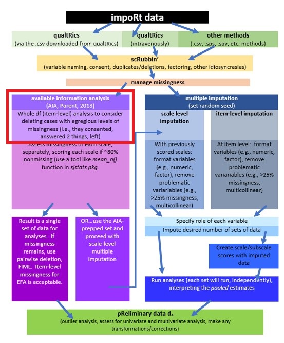
2.4.4 Available Information Analysis (AIA)

Parent (2013) has created a set of recommendations that help us create a streamlined workflow for managing missing data. After evaluating three approaches to managing missingness (AIA, mean substitution, and multiple imputation) Parent concluded that in datasets with (a) low levels of missingness, (b) a reasonable sample size, and (c) adequate internal reliability of measures, these approaches had similar results.

Further, in simulation studies where there was (a) low sample size (n = 50), (b) weak associations among items, and (c) a small number of missing items, AIA was equivalent to multiple imputation. Even in cases where the data conditions were the “best” (i.e., N = 200, moderate correlations, at least 10 items), even 10% missingness (overall) did not produce notable difference among the methods. That is, means, standard errors, and alphas were similar across the methods (AIA, mean substitution, multiple imputation).

AIA is an older method of handling missing data that, as its name suggests, uses the available data for analysis and excludes missing data points only for analyses in which the missing data point would be directly involved. This means

In the case of research that uses multiple item scales, and analysis takes place at the scale level
- AIA is used to generate mean scores for the scale using the available data without substituting or imputing values;
- This method generally produces a fairly complete set of scale-level data where
  - pairwise deletion (the whole row/case/person is skipped) can be used where there will be multiple analyses using statistics (e.g., correlations, t-tests, ANOVA) were missingness is not permitted
  - FIML can be specified in path analysis and CFA/SEM (where item-level data is required), and
  - some statistics, such as principal components analysis and principal axis factoring (item-level analyses) permit missing data,
- Of course, the researcher could still impute data, but why…

Parent’s (2013) recommendations:

Scale scores should be first calculated as a mean (average) not a sum. Why?
- Calculating a “sum” from available data will result in automatically lower scores in cases where there is missingness.
- If a sum is required (i.e., because you want to interpret some clinical level of something), calculate the mean first, do the analyses, then transform the results back into the whole-scale equivalent (multiply the mean by the number of items) for any interpretation.
- For R script, do not write the script ([item1 + item2 + item3]/3) because this will return an empty entry for participants missing data (same problem as if you were to use sum). There are several functions for properly computing a mean; I will demo the mean_n() function from sjstats package because it allows us to simultaneously specify the tolerance level (next item).
Determine your tolerance for missingness (20% seems to be common, although you could also look for guidance in the test manual/article). Then
- Run a “percent missingness” check on the level of analysis (i.e., total score, scale, or subscale) you are using. If you are using a total scale score, then check to see what percent is missing across all the items in the whole scale. In contrast, if you are looking at subscales, run the percent missing at that level.
- Parent (2013) advised that the tolerance levels should be made mindfully. A four-item scale with one item missing, won’t meet the 80% threshold, so it may make sense to set a 75% threshold for this scale.
“Clearly and concisely detail the level of missingness” in papers (Parent, 2013, p. 595). This includes
- tolerance level for missing data by scale or subscale (e.g., 80% or 75%)
- the number of missing values out of all data points on that scale for all participants and the maximum by participant (e.g., “For Scale X, a total of # missing data points out of ### were observed with no participant missing more than a single point.”)
- verify a manual inspection of missing data for obvious patterns (e.g., abnormally high missing rates for only one or two items). This can be accomplished by requesting frequency output for the items and checking the nonmissing data points for each scale, ensuring there are no abnormal spikes in missingness (looking for MNAR).
Curiously, Parent (2013) does not recommend that we run all the diagnostic tests. However, because recent reviewers have required them of me, I will demonstrate a series of them.
Reducing missingness starts at the survey design – make sure that all people can answer all items (i.e,. relationship-related items may contain heterosexist assumptions…which would result in an MNAR circumstance)

Very practically speaking, Parent’s (2013) recommendations follow us through the entire data analysis process.

2.5 Working the Problem

2.5.1 Variable Planning and Preparation

In the Scrubbing lesson we imported the data from Qualtrics and applied the broadest levels of inclusion (e.g., the course rated was offered from an institution in the U.S., the respondent consented to participation) and exclusion (e.g., the survey was not a preview). We then downsized the survey to include the variables we will use in our statistical model. We then saved the data in .csv and .rds file.

Presuming that you are working along with me in an .rmd file and have placed that file in the same folder as this .rmd file, the following code should read the data into your environment.

I use different names for the object/df in my R environment than I use for the filename that holds the data on my computer. Why? I don’t want to accidentally overwrite this precious “source” of data.

# scrub_df <- read.csv ('BlackStntsModel230902.csv', head = TRUE, sep
# = ',')
scrub_df <- readRDS("BlackStntsModel230902.rds")
str(scrub_df)

## Classes 'tbl_df', 'tbl' and 'data.frame':    69 obs. of  25 variables:
##  $ ID       : int  1 2 3 4 5 6 7 8 9 10 ...
##  $ iRace1   : num  3 3 3 3 1 3 3 3 1 0 ...
##   ..- attr(*, "label")= Named chr "1 - From your perspective as a student, which of the following best describes the [Field-2] instructor."
##   .. ..- attr(*, "names")= chr "1_iRace"
##  $ iRace2   : num  1 NA 1 1 NA NA 3 NA NA 0 ...
##   ..- attr(*, "label")= Named chr "2 - From your perspective as a student, which of the following best describes the [Field-2] instructor."
##   .. ..- attr(*, "names")= chr "2_iRace"
##  $ iRace3   : num  3 NA NA 3 NA NA NA NA NA 3 ...
##   ..- attr(*, "label")= Named chr "3 - From your perspective as a student, which of the following best describes the [Field-2] instructor."
##   .. ..- attr(*, "names")= chr "3_iRace"
##  $ iRace4   : num  NA NA NA NA NA NA NA NA NA 3 ...
##   ..- attr(*, "label")= Named chr "4 - From your perspective as a student, which of the following best describes the [Field-2] instructor."
##   .. ..- attr(*, "names")= chr "4_iRace"
##  $ iRace5   : logi  NA NA NA NA NA NA ...
##   ..- attr(*, "label")= Named chr "5 - From your perspective as a student, which of the following best describes the [Field-2] instructor."
##   .. ..- attr(*, "names")= chr "5_iRace"
##  $ iRace6   : logi  NA NA NA NA NA NA ...
##   ..- attr(*, "label")= Named chr "6 - From your perspective as a student, which of the following best describes the [Field-2] instructor."
##   .. ..- attr(*, "names")= chr "6_iRace"
##  $ iRace7   : logi  NA NA NA NA NA NA ...
##   ..- attr(*, "label")= Named chr "7 - From your perspective as a student, which of the following best describes the [Field-2] instructor."
##   .. ..- attr(*, "names")= chr "7_iRace"
##  $ iRace8   : logi  NA NA NA NA NA NA ...
##   ..- attr(*, "label")= Named chr "8 - From your perspective as a student, which of the following best describes the [Field-2] instructor."
##   .. ..- attr(*, "names")= chr "8_iRace"
##  $ iRace9   : logi  NA NA NA NA NA NA ...
##   ..- attr(*, "label")= Named chr "9 - From your perspective as a student, which of the following best describes the [Field-2] instructor."
##   .. ..- attr(*, "names")= chr "9_iRace"
##  $ iRace10  : logi  NA NA NA NA NA NA ...
##   ..- attr(*, "label")= Named chr "10 - From your perspective as a student, which of the following best describes the [Field-2] instructor."
##   .. ..- attr(*, "names")= chr "10_iRace"
##  $ cmBiMulti: num  0 0 0 2 5 15 0 0 0 7 ...
##   ..- attr(*, "label")= Named chr "Regarding race, what proportion of students were from each broad classification.  Your responses should add to "| __truncated__
##   .. ..- attr(*, "names")= chr "Race_10"
##  $ cmBlack  : num  0 5 10 6 5 20 0 0 0 4 ...
##   ..- attr(*, "label")= Named chr "Regarding race, what proportion of students were from each broad classification.  Your responses should add to 100%. - Black"
##   .. ..- attr(*, "names")= chr "Race_1"
##  $ cmNBPoC  : num  39 10 30 19 10 30 40 5 30 13 ...
##   ..- attr(*, "label")= Named chr "Regarding race, what proportion of students were from each broad classification.  Your responses should add to "| __truncated__
##   .. ..- attr(*, "names")= chr "Race_7"
##  $ cmWhite  : num  61 85 60 73 80 35 60 90 70 73 ...
##   ..- attr(*, "label")= Named chr "Regarding race, what proportion of students were from each broad classification.  Your responses should add to 100%. - White"
##   .. ..- attr(*, "names")= chr "Race_8"
##  $ cmUnsure : num  0 0 0 0 0 0 0 5 0 3 ...
##   ..- attr(*, "label")= Named chr "Regarding race, what proportion of students were from each broad classification.  Your responses should add to 100%. - Unsure"
##   .. ..- attr(*, "names")= chr "Race_2"
##  $ Belong_1 : num  6 4 NA 5 4 5 6 7 6 3 ...
##   ..- attr(*, "label")= Named chr "Please indicate the degree to which you agree with the following questions about the course. Please skip the it"| __truncated__
##   .. ..- attr(*, "names")= chr "Belong_1"
##  $ Belong_2 : num  6 4 3 3 4 6 6 7 6 3 ...
##   ..- attr(*, "label")= Named chr "Please indicate the degree to which you agree with the following questions about the course. Please skip the it"| __truncated__
##   .. ..- attr(*, "names")= chr "Belong_2"
##  $ Belong_3 : num  7 6 NA 2 4 5 5 7 6 3 ...
##   ..- attr(*, "label")= Named chr "Please indicate the degree to which you agree with the following questions about the course. Please skip the it"| __truncated__
##   .. ..- attr(*, "names")= chr "Belong_3"
##  $ Blst_1   : num  5 6 NA 2 6 5 5 5 5 3 ...
##   ..- attr(*, "label")= Named chr "Each item below asks you to rate elements of campus climate for your \"academic department/program.\"  If you d"| __truncated__
##   .. ..- attr(*, "names")= chr "Blst_1"
##  $ Blst_2   : num  3 6 5 2 1 1 4 4 3 5 ...
##   ..- attr(*, "label")= Named chr "Each item below asks you to rate elements of campus climate for your \"academic department/program.\"  If you d"| __truncated__
##   .. ..- attr(*, "names")= chr "Blst_2"
##  $ Blst_3   : num  5 2 2 2 1 1 4 3 1 2 ...
##   ..- attr(*, "label")= Named chr "Each item below asks you to rate elements of campus climate for your \"academic department/program.\"  If you d"| __truncated__
##   .. ..- attr(*, "names")= chr "Blst_3"
##  $ Blst_4   : num  2 2 2 2 1 2 4 3 2 3 ...
##   ..- attr(*, "label")= Named chr "Each item below asks you to rate elements of campus climate for your \"academic department/program.\"  If you d"| __truncated__
##   .. ..- attr(*, "names")= chr "Blst_4"
##  $ Blst_5   : num  2 4 NA 2 1 1 4 4 1 3 ...
##   ..- attr(*, "label")= Named chr "Each item below asks you to rate elements of campus climate for your \"academic department/program.\"  If you d"| __truncated__
##   .. ..- attr(*, "names")= chr "Blst_5"
##  $ Blst_6   : num  2 1 2 2 1 2 4 3 2 3 ...
##   ..- attr(*, "label")= Named chr "Each item below asks you to rate elements of campus climate for your \"academic department/program.\"  If you d"| __truncated__
##   .. ..- attr(*, "names")= chr "Blst_6"
##  - attr(*, "column_map")=Classes 'tbl_df', 'tbl' and 'data.frame':   182 obs. of  7 variables:
##   ..$ qname      : chr [1:182] "StartDate" "EndDate" "Status" "Progress" ...
##   ..$ description: chr [1:182] "Start Date" "End Date" "Response Type" "Progress" ...
##   ..$ main       : chr [1:182] "Start Date" "End Date" "Response Type" "Progress" ...
##   ..$ sub        : chr [1:182] "" "" "" "" ...
##   ..$ ImportId   : chr [1:182] "startDate" "endDate" "status" "progress" ...
##   ..$ timeZone   : chr [1:182] "America/Los_Angeles" "America/Los_Angeles" NA NA ...
##   ..$ choiceId   : chr [1:182] NA NA NA NA ...

Let’s think about how the variables in our model should be measured:

DV: Campus Climate for Black Students (as perceived by the respondent)
- mean score of the 6 items on that scale (higher scores indicate a climate characterized by hostility, nonresponsiveness, and stigma)
- 1 item needs to be reverse-coded
- this scale was adapted from the LGBT Campus Climate Scale (Szymanski & Bissonette, 2020)
IV: Belonging
- mean score for the 3 items on that scale (higher scores indicate a greater sense of belonging)
- this scale is taken from the Sense of Belonging subscale from the Perceived Cohesion Scale (Bollen & Hoyle, 1990)
Proportion of classmates who are Black
- a single item
Proportion of instructional staff who are BIPOC
- must be calculated from each of the single items for each instructor

To summarize, the Campus Climate and Belonging scales are traditional in the sense that they have items that we sum. The variable representing proportion of classmates who are Black is a single item. The variable representing the proportion of instructional staff who are BIPOC must be calculated in a manner that takes into consideration the there may be multiple instructors. The survey allowed a respondent to name up to 10 instructors.

str(scrub_df$iRace1)

##  num [1:69] 3 3 3 3 1 3 3 3 1 0 ...
##  - attr(*, "label")= Named chr "1 - From your perspective as a student, which of the following best describes the [Field-2] instructor."
##   ..- attr(*, "names")= chr "1_iRace"

Looking at the structure of our data, the iRace(1 thru 10) variables are in “int” or integer format. This means that they are represented as whole numbers. We need them to be represented as factors. R handles factors represented as words well. Therefore, let’s use our codebook to reformat this variable as a an ordered factor, with words instead of numbers.

Qualtrics imports many of the categorical variables as numbers. R often reads them numerically (integers or numbers). If they are directly converted to factors, R will sometimes collapse across missing numbers. In this example, if there is a race that is not represented (e.g., 2 for BiMulti), when the numbers are changed to factors, R will assume they are ordered and there is a consecutive series of numbers (0,1,2,3,4). If a number in the sequence is missing (0,1,3,4) and labels are applied, it will collapse across the numbers and the labels you think are attached to each number are not. Therefore, it is ESSENTIAL to check (again and again ad nauseum) to ensure that your variables are recoding in a manner you understand.

One way to avoid this is to use the code below to identify the levels and the labels. When they are in order, they align and don’t “skip” numbers. To quadruple check our work, we will recode into a new variable “tRace#” for “teacher” Race.

scrub_df$tRace1 = factor(scrub_df$iRace1, levels = c(0, 1, 2, 3, 4), labels = c("Black",
    "nBpoc", "BiMulti", "White", "NotNotice"))
scrub_df$tRace2 = factor(scrub_df$iRace2, levels = c(0, 1, 2, 3, 4), labels = c("Black",
    "nBpoc", "BiMulti", "White", "NotNotice"))
scrub_df$tRace3 = factor(scrub_df$iRace3, levels = c(0, 1, 2, 3, 4), labels = c("Black",
    "nBpoc", "BiMulti", "White", "NotNotice"))
scrub_df$tRace4 = factor(scrub_df$iRace4, levels = c(0, 1, 2, 3, 4), labels = c("Black",
    "nBpoc", "BiMulti", "White", "NotNotice"))
scrub_df$tRace5 = factor(scrub_df$iRace5, levels = c(0, 1, 2, 3, 4), labels = c("Black",
    "nBpoc", "BiMulti", "White", "NotNotice"))
scrub_df$tRace6 = factor(scrub_df$iRace6, levels = c(0, 1, 2, 3, 4), labels = c("Black",
    "nBpoc", "BiMulti", "White", "NotNotice"))
scrub_df$tRace7 = factor(scrub_df$iRace7, levels = c(0, 1, 2, 3, 4), labels = c("Black",
    "nBpoc", "BiMulti", "White", "NotNotice"))
scrub_df$tRace8 = factor(scrub_df$iRace8, levels = c(0, 1, 2, 3, 4), labels = c("Black",
    "nBpoc", "BiMulti", "White", "NotNotice"))
scrub_df$tRace9 = factor(scrub_df$iRace9, levels = c(0, 1, 2, 3, 4), labels = c("Black",
    "nBpoc", "BiMulti", "White", "NotNotice"))
scrub_df$tRace10 = factor(scrub_df$iRace10, levels = c(0, 1, 2, 3, 4),
    labels = c("Black", "nBpoc", "BiMulti", "White", "NotNotice"))

Let’s check the structure to see if they are factors.

library(tidyverse)

## ── Attaching core tidyverse packages ──────────────────────── tidyverse 2.0.0 ──
## ✔ dplyr     1.1.2     ✔ readr     2.1.4
## ✔ forcats   1.0.0     ✔ stringr   1.5.1
## ✔ ggplot2   3.5.0     ✔ tibble    3.2.1
## ✔ lubridate 1.9.2     ✔ tidyr     1.3.0
## ✔ purrr     1.0.1     
## ── Conflicts ────────────────────────────────────────── tidyverse_conflicts() ──
## ✖ dplyr::filter() masks stats::filter()
## ✖ dplyr::lag()    masks stats::lag()
## ℹ Use the conflicted package (<http://conflicted.r-lib.org/>) to force all conflicts to become errors

glimpse(scrub_df)

## Rows: 69
## Columns: 35
## $ ID        <int> 1, 2, 3, 4, 5, 6, 7, 8, 9, 10, 11, 12, 13, 14, 15, 16, 17, 1…
## $ iRace1    <dbl> 3, 3, 3, 3, 1, 3, 3, 3, 1, 0, 2, 1, 1, 1, 3, 3, 3, 1, 3, 3, …
## $ iRace2    <dbl> 1, NA, 1, 1, NA, NA, 3, NA, NA, 0, NA, NA, 3, NA, 3, 3, NA, …
## $ iRace3    <dbl> 3, NA, NA, 3, NA, NA, NA, NA, NA, 3, NA, NA, NA, NA, 3, 1, N…
## $ iRace4    <dbl> NA, NA, NA, NA, NA, NA, NA, NA, NA, 3, NA, NA, NA, NA, NA, 3…
## $ iRace5    <lgl> NA, NA, NA, NA, NA, NA, NA, NA, NA, NA, NA, NA, NA, NA, NA, …
## $ iRace6    <lgl> NA, NA, NA, NA, NA, NA, NA, NA, NA, NA, NA, NA, NA, NA, NA, …
## $ iRace7    <lgl> NA, NA, NA, NA, NA, NA, NA, NA, NA, NA, NA, NA, NA, NA, NA, …
## $ iRace8    <lgl> NA, NA, NA, NA, NA, NA, NA, NA, NA, NA, NA, NA, NA, NA, NA, …
## $ iRace9    <lgl> NA, NA, NA, NA, NA, NA, NA, NA, NA, NA, NA, NA, NA, NA, NA, …
## $ iRace10   <lgl> NA, NA, NA, NA, NA, NA, NA, NA, NA, NA, NA, NA, NA, NA, NA, …
## $ cmBiMulti <dbl> 0, 0, 0, 2, 5, 15, 0, 0, 0, 7, 0, 0, 20, 0, 9, 12, 0, 6, 6, …
## $ cmBlack   <dbl> 0, 5, 10, 6, 5, 20, 0, 0, 0, 4, 0, 7, 0, 6, 9, 1, 21, 5, 6, …
## $ cmNBPoC   <dbl> 39, 10, 30, 19, 10, 30, 40, 5, 30, 13, 80, 19, 0, 19, 15, 22…
## $ cmWhite   <dbl> 61, 85, 60, 73, 80, 35, 60, 90, 70, 73, 10, 74, 80, 0, 67, 5…
## $ cmUnsure  <dbl> 0, 0, 0, 0, 0, 0, 0, 5, 0, 3, 10, 0, 0, 75, 0, 14, 0, 5, 0, …
## $ Belong_1  <dbl> 6, 4, NA, 5, 4, 5, 6, 7, 6, 3, 6, 6, 3, 4, 3, 3, 4, 5, 1, 2,…
## $ Belong_2  <dbl> 6, 4, 3, 3, 4, 6, 6, 7, 6, 3, 6, 6, 5, 4, 3, 3, 4, 6, 1, 2, …
## $ Belong_3  <dbl> 7, 6, NA, 2, 4, 5, 5, 7, 6, 3, 5, 6, 4, 4, 3, 2, 4, 5, 1, 1,…
## $ Blst_1    <dbl> 5, 6, NA, 2, 6, 5, 5, 5, 5, 3, NA, 4, 5, 6, 3, 4, 6, 4, 4, 4…
## $ Blst_2    <dbl> 3, 6, 5, 2, 1, 1, 4, 4, 3, 5, NA, 5, 1, 1, 3, 2, 1, 2, 5, 3,…
## $ Blst_3    <dbl> 5, 2, 2, 2, 1, 1, 4, 3, 1, 2, 2, 1, 1, 1, 3, 2, 6, 2, 2, 2, …
## $ Blst_4    <dbl> 2, 2, 2, 2, 1, 2, 4, 3, 2, 3, NA, 4, 3, 1, 3, 2, 1, 3, 2, 1,…
## $ Blst_5    <dbl> 2, 4, NA, 2, 1, 1, 4, 4, 1, 3, 2, 2, 1, 1, 3, 2, 1, 2, 2, 1,…
## $ Blst_6    <dbl> 2, 1, 2, 2, 1, 2, 4, 3, 2, 3, NA, 2, 1, 1, 3, 2, 2, 3, 2, 1,…
## $ tRace1    <fct> White, White, White, White, nBpoc, White, White, White, nBpo…
## $ tRace2    <fct> nBpoc, NA, nBpoc, nBpoc, NA, NA, White, NA, NA, Black, NA, N…
## $ tRace3    <fct> White, NA, NA, White, NA, NA, NA, NA, NA, White, NA, NA, NA,…
## $ tRace4    <fct> NA, NA, NA, NA, NA, NA, NA, NA, NA, White, NA, NA, NA, NA, N…
## $ tRace5    <fct> NA, NA, NA, NA, NA, NA, NA, NA, NA, NA, NA, NA, NA, NA, NA, …
## $ tRace6    <fct> NA, NA, NA, NA, NA, NA, NA, NA, NA, NA, NA, NA, NA, NA, NA, …
## $ tRace7    <fct> NA, NA, NA, NA, NA, NA, NA, NA, NA, NA, NA, NA, NA, NA, NA, …
## $ tRace8    <fct> NA, NA, NA, NA, NA, NA, NA, NA, NA, NA, NA, NA, NA, NA, NA, …
## $ tRace9    <fct> NA, NA, NA, NA, NA, NA, NA, NA, NA, NA, NA, NA, NA, NA, NA, …
## $ tRace10   <fct> NA, NA, NA, NA, NA, NA, NA, NA, NA, NA, NA, NA, NA, NA, NA, …

Calculating the proportion of the BIPOC instructional staff could likely be accomplished a number of ways. My searching for solutions resulted in this. Hopefully it’s a fair balance between intuitive and elegant coding. First, I created code that

created a new variable (count.BIPOC) by
- summing across the tRace1 through tRace10 variables,
- assigning a count of “1” each time the factor value was Black, nBpoc, or BiMulti

scrub_df$count.BIPOC <- apply(scrub_df[c("tRace1", "tRace2", "tRace3",
    "tRace4", "tRace5", "tRace6", "tRace7", "tRace8", "tRace9", "tRace10")],
    1, function(x) sum(x %in% c("Black", "nBpoc", "BiMulti")))

Next, I created a variable that counted the number of non-missing values across the tRace1 through tRace10 variables.

scrub_df$count.nMiss <- apply(scrub_df[c("tRace1", "tRace2", "tRace3",
    "tRace4", "tRace5", "tRace6", "tRace7", "tRace8", "tRace9", "tRace10")],
    1, function(x) sum(!is.na(x)))

Now to calculate the proportion of BIPOC instructional faculty for each case.

scrub_df$iBIPOC_pr = scrub_df$count.BIPOC/scrub_df$count.nMiss

2.5.2 Missing Data Analysis: Whole df and Item level

In understanding missingness across the dataset, I think it is important to analyze and manage it, iteratively. We will start with a view of the whole df-level missingness. Subsequently, and consistent with the available information analysis [AIA; Parent (2013)] approach, we will score the scales and then look again at missingness, using the new information to update our decisions about how to manage it.

An image of our stage in the workflow for scrubbing and scoring data.

Because we just created a host of new variables in creating the prop_BIPOC variable, let’s downsize the df so that the calculations are sensible.

scrub_df <- (select(scrub_df, ID, iBIPOC_pr, cmBlack, Belong_1:Belong_3,
    Blst_1:Blst_6))

With a couple of calculations, we create a proportion of item-level missingness.

In this chunk I first calculate the number of missing (nmiss)

library(tidyverse)
#Calculating number and proportion of item-level missingness
scrub_df$nmiss <- scrub_df%>%
    select(iBIPOC_pr:Blst_6) %>% #the colon allows us to include all variables between the two listed (the variables need to be in order)
    is.na %>% 
    rowSums

scrub_df<- scrub_df%>%
  dplyr::mutate(prop_miss = (nmiss/11)*100) #11 is the number of variables included in calculating the proportion

We can grab the descriptives for the prop_miss variable to begin to understand our data. I will create an object from it so I can use it with inline

psych::describe(scrub_df$prop_miss)

##    vars  n mean    sd median trimmed mad min max range skew kurtosis   se
## X1    1 69 7.77 22.61      0    1.59   0   0 100   100 3.04     8.19 2.72

CUMULATIVE CAPTURE FOR WRITING IT UP:

Across cases that were deemed eligible on the basis of the inclusion/exclusion criteria, missingness ranged from 0 to 100%.

At the time that I am lecturing this, we do have some rather egregious missingness. At this point I will write code to eliminate cases with \(\geq\) 90%.

scrub_df <- dplyr::filter(scrub_df, prop_miss <= 90)  #update df to have only those with at least 90% of complete data

To analyze missingness at this level, we need a df that has only the variables of interest. That is, variables like ID and the prop_miss and nmiss variables we created will interfere with an accurate assessment of missingness. I will update our df to eliminate these.

# further update to exclude the n_miss and prop_miss variables
scrub_df <- scrub_df %>%
    dplyr::select(-c(ID, nmiss, prop_miss))

Missing data analysis commonly looks at proportions by:

the entire df
rows/cases/people

# what proportion of cells missing across entire dataset
formattable::percent(mean(is.na(scrub_df)))

## [1] 3.86%

# what proportion of cases (rows) are complete (nonmissing)
formattable::percent(mean(complete.cases(scrub_df)))

## [1] 87.88%

CUMULATIVE CAPTURE FOR WRITING IT UP:

Across cases that were deemed eligible on the basis of the inclusion/exclusion criteria, missingness ranged from 0 to 100%. Across the dataset, 3.86% of cells had missing data and 87.88% of cases had nonmissing data.

2.5.3 Analyzing Missing Data Patterns

One approach to analyzing missing data is to assess patterns of missingness.

Several R packages are popularly used for conducting such analyses. In the mice package, md.pattern() function provides a matrix with the number of columns + 1, in which each row corresponds to a missing data pattern (1 = observed, 0 = missing).

Rows and columns are sorted in increasing amounts of missing information.

The last column and row contain row and column counts, respectively.

mice_out <- mice::md.pattern(scrub_df, plot = TRUE, rotate.names = TRUE)
mice_out
write.csv(mice_out, file = "mice_out.csv")  #optional to write it to a .csv file

The table lets us examine each missing pattern and see which variable(s) is/are missing. The output is in the form of a table that indicates the frequency of each pattern of missingness. Because I haven’t (yet) figured out how to pipe objects from this table into the chapter, this text may differ from the patterns in the current data frame.

Each row in the table represents a different pattern of missingness. At the time of writing, there are 8 patterns of missing data. The patterns are listed in descending order of the least amount of missingness. The most common pattern (58 cases, top row) is one with no missing data. One case is missing one cell – one item assessing the campus climate for Black students, and so forth.

2.5.4 Can we identify the missing mechanisms?

To date, we do not have statistical tools that can accurately diagnose our patterns of missingness. You may have heard that “Little’s MCAR” is a helpful tool. Unfortunately, as Enders (2010) has noted, the tool is problematic. Perhaps the most significant one is that under the null hypothesis, a statistically significant test indicates that the missing data are MAR (missing at random) or MNAR (missing not at random); a non-significant test indicates the data are MCAR (missing completely at random) or MNAR. Consequently, regardless of the result, an MNAR circumstance cannot be ruled out. Correspondingly, the Little’s MCAR test has disappeared from the more reliable R packages that assess missingness.

Enders (2010) Applied Missing Data Analysis text does provide a set of figures (page 3) that illustrate common missing data patterns. Comparing these to the figure produced with mice::mdpattern our data looks somewhat monotonic – that is, as individuals completed the survey, they began to experience test fatigue and simply stopped responding. Diagnosisng monotonicity requires that the variables in the dataset must be in the order in which the students completed them. If the variables have been re-ordered or if the surveys were presented to students in a randomized order, then more data manipulation would be required before attributing missingness to test fatigue.

Survey programs like Qualtrics offer the randomization of items within blocks (or blocks themselves). This can help distribute missingness caused by test fatigue so that more cases can be retained.

2.6 Scoring

So let’s get to work to score up the measures for our analysis. Each step of this should involve careful cross-checking with the codebook.

2.6.1 Reverse scoring

As we discovered previously, in the scale that assesses campus climate (higher scores reflect a more negative climate) one of our items (Blst_1, “My institution provides a supportive environment for Black students.”) requires reverse-coding.

To rescore:

Create a new variable (this is essential) that is designated as the reversed item. We might put a the letter “r” (for reverse scoring) at the beginning or end: rBlst_1 or Blst_1r. It does not matter; just be consistent.
- We don’t reverse score into the same variable because when you rerun the script, it just re-reverses the reversed score…into infinity. It’s very easy to lose your place.
The reversal is an equation where you subtract the value in the item from the range/scaling + 1. For the our three items we subtract each item’s value from 8.

scrub_df <- scrub_df %>%
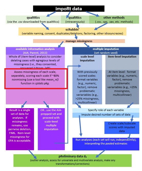
    dplyr::mutate(rBlst_1 = 8 - Blst_1)  #if you had multiple items, you could add a pipe (%>%) at the end of the line and add more until the last one

Per Parent (2013) we will analyze missingness for each scale, separately.

We will calculate scale scores on each scale separately when 80% (roughly) of the data is present.
- this is somewhat arbitrary, on 4 item scales, I would choose 75% (to allow one to be missing)
- on the 3 item scale, I will allow one item to be missing (65%)
After calculating the scale scores, we will return to analyzing the missingness, looking at the whole df

The mean_n() function of sjstats package has allows you to specify how many items (whole number) or what percentage of items should be present in order to get the mean. First, though, we should identify the variables (properly formatted, if rescoring was needed) that should be included in the calculation of each scale and subscale.

In our case, the scale assessing belonging (Bollen & Hoyle, 1990; Hurtado & Carter, 1997) involves three items with no reversals. Our campus climate scale was adapted from Szymanski et al.’s LGBTQ College Campus Climate Scale (Szymanski & Bissonette, 2020). While it has not been psychometrically evaluated for the purpose for which I am using it, I will follow the scoring structure in the journal article that introduces the measure. Specifically, the factor structure permits a total scale score and two subscales representing the college response and stigma.

# Making the list of variables
Belonging_vars <- c("Belong_1", "Belong_2", "Belong_3")
ResponseBL_vars <- c("rBlst_1", "Blst_4", "Blst_6")
StigmaBL_vars <- c("Blst_2", "Blst_3", "Blst_5")
ClimateBL_vars <- c("rBlst_1", "Blst_4", "Blst_6", "Blst_2", "Blst_3",
    "Blst_5")

# Creating the new variables
scrub_df$Belonging <- sjstats::mean_n(scrub_df[, Belonging_vars], 0.65)
scrub_df$ResponseBL <- sjstats::mean_n(scrub_df[, ResponseBL_vars], 0.8)
scrub_df$StigmaBL <- sjstats::mean_n(scrub_df[, StigmaBL_vars], 0.8)
scrub_df$ClimateBL <- sjstats::mean_n(scrub_df[, ClimateBL_vars], 0.8)

# If the scoring code above does not work for you, try the format
# below which involves inserting to periods in front of the variable
# list. One example is provided. dfLewis$Belonging <-
# sjstats::mean_n(dfLewis[, ..Belonging_vars], 0.80)

Later it will be helpful to have a df with the item and scale-level variables. It will also be helpful if there is an ID for each case.

scrub_df <- scrub_df %>%
    dplyr::mutate(ID = row_number())

# moving the ID number to the first column; requires
scrub_df <- scrub_df %>%
    dplyr::select(ID, everything())

Let’s save our scrub_df data for this and write it as an outfile. I will save it in both .rds and .csv formats so that you can use either one.

write.table(scrub_df, file = "BlStItmsScrs230902.csv", sep = ",", col.names = TRUE,
    row.names = FALSE)
saveRDS(scrub_df, "BlStItmsScrs230902.rds")

2.7 Missing Analysis: Scale level

Let’s return to analyzing the missingness, this time including the scale level variables (without the individual items) that will be in our statistical model(s).

An image of our stage in the workflow for scrubbing and scoring data.

First let’s get the df down to the variables we want to retain:

scored <- dplyr::select(scrub_df, iBIPOC_pr, cmBlack, Belonging, ResponseBL,
    StigmaBL, ClimateBL)
ScoredCaseMiss <- nrow(scored)  #I produced this object for the sole purpose of feeding the number of cases into the inline text, below
ScoredCaseMiss

## [1] 66

Before we start our formal analysis of missingness at the scale level, let’s continue to scrub by eliminating cases that will have too much missingness. In the script below we create a variable that counts the number of missing variables and then creates a proportion by dividing it by the number of total variables.

Using the describe() function from the psych package, we can investigate this variable.

# Create a variable (n_miss) that counts the number missing
scored$n_miss <- scored %>%
    dplyr::select(iBIPOC_pr:ClimateBL) %>%
    is.na %>%
    rowSums

# Create a proportion missing by dividing n_miss by the total number
# of variables (6) Pipe to sort in order of descending frequency to
# get a sense of the missingness
scored <- scored %>%
    dplyr::mutate(prop_miss = (n_miss/6) * 100) %>%
    arrange(desc(n_miss))

psych::describe(scored$prop_miss)

##    vars  n mean    sd median trimmed mad min   max range skew kurtosis   se
## X1    1 66 3.79 12.33      0    0.31   0   0 66.67 66.67 3.44    11.77 1.52

CUMULATIVE CAPTURE FOR WRITING IT UP:

Across cases that were deemed eligible on the basis of the inclusion/exclusion criteria, missingness ranged from 0 to 100%. Across the dataset, 3.86% of cells had missing data and 87.88% of cases had nonmissing data.

Across the 66 cases for which the scoring protocol was applied, missingness ranged from 0 to 67%.

We need to decide what is our retention threshhold. Twenty percent seems to be a general rule of thumb. Let’s delete all cases with missingness at 20% or greater.

# update df to have only those with at least 20% of complete data
# (this is an arbitrary decision)
scored <- dplyr::filter(scored, prop_miss <= 20)

# the variable selection just lops off the proportion missing
scored <- (select(scored, iBIPOC_pr:ClimateBL))

# this produces the number of cases retained
nrow(scored)

## [1] 61

CUMULATIVE CAPTURE FOR WRITING IT UP:

Across cases that were deemed eligible on the basis of the inclusion/exclusion criteria, missingness ranged from 0 to 100%. Across the dataset, 3.86% of cells had missing data and 87.88% of cases had nonmissing data.

Across the 66 cases for which the scoring protocol was applied, missingness ranged from 0 to 67%. After eliminating cases with greater than 20% missing, the dataset analyzed included 61 cases.

With a decision about the number of cases we are going to include, we can continue to analyze missingness.

2.8 Revisiting Missing Analysis at the Scale Level

We work with a df that includes only the variables in our model. In our case this is easy. In other cases (i.e., maybe there is an ID number) it might be good to create a subset just for this analysis.

Again, we look at missingness as the proportion of

individual cells across the scored dataset, and
rows/cases with nonmissing data

# percent missing across df
formattable::percent(mean(is.na(scored)))

## [1] 0.55%

# percent of rows with nonmissing data
formattable::percent(mean(complete.cases(scored)))

## [1] 96.72%

CUMULATIVE CAPTURE FOR WRITING IT UP:

Across cases that were deemed eligible on the basis of the inclusion/exclusion criteria, missingness ranged from 0 to 100%. Across the dataset, 3.86% of cells had missing data and 87.88% of cases had nonmissing data.

Across the 66 cases for which the scoring protocol was applied, missingness ranged from 0 to 67%. After eliminating cases with greater than 20% missing, the dataset analyzed included 61 cases. In this dataset we had less than 1% (0.55%) missing across the df; 97% of the rows had nonmissing data.

Let’s look again at missing patterns and mechanisms.

2.8.1 Scale Level: Patterns of Missing Data

Returning to the mice package, we can use the md.pattern() function to examine a matrix with the number of columns + 1 in which each row corresponds to a missing data pattern (1 = observed, 0 = missing). The rows and columns are sorted in increasing amounts of missing information. The last column and row contain row and column counts, respectively.

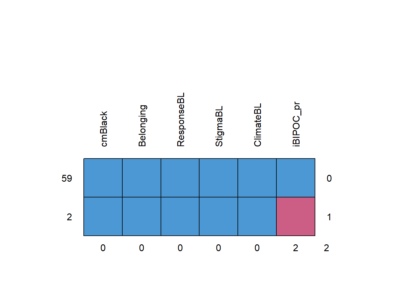
mice_ScaleLvl <- mice::md.pattern(scored, plot = TRUE, rotate.names = TRUE)

mice_ScaleLvl

##    cmBlack Belonging ResponseBL StigmaBL ClimateBL iBIPOC_pr  
## 59       1         1          1        1         1         1 0
## 2        1         1          1        1         1         0 1
##          0         0          0        0         0         2 2

At the scale-level, this is much easier to interpret. There are 2 rows of data because there are only 2 patterns of missingness. The most common pattern is non-missing data (n = 59).

If our statistical choice uses listwise deletion (i.e., the case is eliminated if one or more variables in the model has missing data), our sample size will be 59. As we will earn in later chapters, there are alternatives (i.e., specifying a FIML option in analyses that use maximum likelihood estimators) that can use all of the cases – even those with missing data.

2.8.2 R-eady for Analysis

At this stage the data is ready for analysis (data diagnostics). With the AIA approach (Parent, 2013) the following preliminary analyses would involve pairwise deletion (i.e., the row/case is dropped for that analysis, but included for all others):

An image of our stage in the workflow for scrubbing and scoring data.

data diagnostics
- psychometric properties of scales, such as alpha coefficients
- assessing assumptions such as univariate and multivariate normality, outliers, etc.
preliminary analyses
- descriptives (means/standard deviations, frequencies)
- correlation matrices

AIA can also be used with primary analyses. Examples of how to manage missingness include:

ANOVA/regression models
- if completed with ordinary least squares, pairwise deletion would be utilized
SEM/CFA models with observed, latent, or hybrid models
- if FIML (we’ll discuss later) is specified, all cases are used, even when there is missingness
EFA models
- these can handle item-level missingness
Hierarchical linear modeling/multilevel modeling/mixed effects modeling
- While all data needs to be present for a given cluster/wave, it is permissible to have varying numbers of clusters/waves per case

2.9 The APA Style Write-Up

2.10 Results

All analyses were completed in R Studio (v. RStudio 2023.06.1+524 “Mountain Hydrangea”) with R (v. 4.3.1).

Missing Data Analysis and Treatment of Missing Data

Available item analysis (AIA; (Parent, 2013)) is a strategy for managing missing data that uses available data for analysis and excludes cases with missing data points only for analyses in which the data points would be directly involved. Parent (2013) suggested that AIA is equivalent to more complex methods (e.g., multiple imputation) across a number of variations of sample size, magnitude of associations among items, and degree of missingness. Thus, we utilized Parent’s recommendations to guide our approach to managing missing data. Missing data analyses were conducted with tools in base R as well as the R packages, psych (v. 2.3.6) and mice (v. 3.16.0).

Across cases that were deemed eligible on the basis of the inclusion/exclusion criteria, missingness ranged from 0 to 67%. Across the dataset, 3.86% of cells had missing data and 87.88% of cases had nonmissing data. At this stage in the analysis, we allowed all cases with less than 90% missing to continue to the scoring stage. Guided by Parent’s (2013) AIA approach, scales with three items were scored if at least two items were non-missing; the scale with four items was scored if it at least three non-missing items; and the scale with six items was scored if it had at least five non-missing items.

Across the 66 cases for which the scoring protocol was applied, missingness ranged from 0 to 67%. After eliminating cases with greater than 20% missing, the dataset analyzed included 61 cases. In this dataset we had less than 1% (0.55%) missing across the data set; 97% of the rows had nonmissing data.

2.11 Practice Problems

The three problems described below are designed to be continuations from the previous chapter (Scrubbing). You will likely encounter challenges that were not covered in this chapter. Search for and try out solutions, knowing that there are multiple paths through the analysis. The overall notion of the suggestions for practice are to (a) properly format three variables, (b) evaluate item-level missingness, (c) score any scales, (c) evaluate scale-level missingness, (d) provide an APA-style write-up, and (e) explain it to someone.

2.11.1 Problem #1: Reworking the Chapter Problem

If you chose this option in the prior chapter, you imported the data from Qualtrics, applied inclusion/exclusion criteria, renamed variables, downsized the df to the variables of interest, and wrote up the preliminary results.

2.11.2 Problem #2: Use the Rate-a-Recent-Course Survey, Choosing Different Variables

If you chose this option in the prior chapter, you chose a minimum of three variables from the Rate-a-Recent-Course survey to include in a simple statistical model. You imported the dat from Qualtrics, applied inclusion/exclusion criteria, renamed variables, downsized the df to the variables of interest and wrote up the preliminary results.

2.11.3 Problem #3: Other data

If you chose this option in the prior chapter, you used raw data that was available to you. You imported it into R, applied inclusion/exclusion criteria, renamed variables, downsized the df to the variables of interest, and wrote up the preliminary results.

2.11.4 Grading Rubric

Assignment Component	Points Possible	Points Earned
1. Proper formatting of the items(s) in your first predictor variable	5	_____
2. Proper formatting of the items(s) in your second predictor variable	5	_____
3. Proper formatting of the items(s) your third predictor variable	5	_____
4. Proper formatting of your dependent variable	5	_____
4. Evaluate and interpret item-level missingness	5	_____
5. Score any scales/subscales	5	_____
7. Represent your work in an APA-style write-up (added to the writeup in the previous chapter)	5	_____
8. Explanation to grader	5	_____
Totals	45	_____

A homeworked example for the Scrubbing, Scoring, and DataDx lessons (combined) follows the Data Dx lesson.

REFERENCES

Bollen, K. A., & Hoyle, R. H. (1990). Perceived cohesion: A conceptual and empirical examination. Social Forces, 69(2), 479–504. https://doi.org/10.2307/2579670

Enders, C. K. (2010). Applied missing data analysis. Guilford Press.

Hurtado, S., & Carter, D. F. (1997). Effects of college transition and perceptions of the campus racial climate on Latino college students’ sense of belonging. Sociology of Education, 70, 324–345. https://doi.org/10.2307/2673270

Kline, R. B. (2016b). Principles and practice of structural equation modeling (4th ed.). Guilford Publications. http://ebookcentral.proquest.com/lib/spu/detail.action?docID=4000663

Little, R. J. A., & Rubin, D. B. (2002). Statistical analysis with missing data (Second edition.). Wiley. http://site.ebrary.com/id/10921256

Parent, M. C. (2013). Handling item-level missing data: Simpler is just as good. The Counseling Psychologist, 41(4), 568–600. https://doi.org/10.1177/0011000012445176

Szymanski, D. M., & Bissonette, D. (2020). Perceptions of the LGBTQ College Campus Climate Scale: Development and psychometric evaluation. Journal of Homosexuality, 67(10), 1412–1428. https://doi.org/10.1080/00918369.2019.1591788