Chapter 4 Multiple Imputation (A Brief Demo)
Multiple imputation is a tool for managing missing data that works with the whole raw data file to impute values for missing data for multiple sets (e.g., 5-20) of the raw data. Those multiple sets are considered together in analyses (such as regression) and interpretation is made on the pooled results. Much has been written about multiple imputation and, if used, should be done with many considerations. This chapter is intended as a brief introduction. In this chapter, I demonstrate the use of multiple imputation with the data from the Rate-a-Recent-Course: A ReCentering Psych Stats Exercise that has served as the research vignette for the first few chapters of this OER.
4.2 Workflow for Multiple Imputation
The following is a proposed workflow for preparing data for analysis.
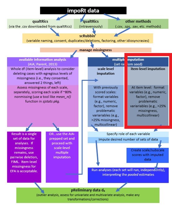
In this lecture we are working on the right side of the flowchart in the multiple imputation (blue) section. Within it, there are two options, each with a slightly different set of options.
- imputing at the item level
- in this case, scales/subscales are scored after the item-level imputation
- imputating at the scale level
- in this case, scales/subscales are scored prior to the imputation; likely using some of the same criteria as identified in the scoring chapter (i.e., scoring if 75-80% of data are non-missing). Multiple imputation, then, is used to estimate the remaining, missing values.
Whichever approach is used, the imputed variables (multiple sets) are used in a pooled analysis and results are interpreted from that analysis.
4.3 Research Vignette
The research vignette comes from the survey titled, Rate-a-Recent-Course: A ReCentering Psych Stats Exercise and is explained in the scrubbing chapter. In the scoring chapter we prepared four variables for analysis. In the data diagnostics chapter we assessed the quality of the variables and conducted the multiple regression described below. Details for these are in our codebook.
Let’s quickly review the variables in our model:
- Perceived Campus Climate for Black Students includes 6 items, one of which was reverse scored. This scale was adapted from Szymanski et al.’s (2020) Campus Climate for LGBTQ students. It has not been evaluated for use with other groups. The Szymanski et al. analysis suggested that it could be used as a total scale score, or divided into three items each that assess
- College response to LGBTQ students (items 6, 4, 1)
- LGBTQ stigma (items 3, 2, 5)
- Sense of Belonging includes 3 items. This is a subscale from Bollen and Hoyle’s (1990) Perceived Cohesion Scale. There are no items on this scale that require reversing.
- Percent of Black classmates is a single item that asked respondents to estimate the proportion of students in various racial categories
- Percent of BIPOC instructional staff, similarly, asked respondents to identify the racial category of each member of their instructional staff
As we noted in the scrubbing chapter, our design has notable limitations. Briefly, (a) owing to the open source aspect of the data we do not ask about the demographic characteristics of the respondent; (b) the items that ask respondents to guess the identities of the instructional staff and to place them in broad categories, (c) we do not provide a “write-in” a response. We made these decisions after extensive conversation with stakeholders. The primary reason for these decisions was to prevent potential harm (a) to respondents who could be identified if/when the revealed private information in this open-source survey, and (b) trolls who would write inappropriate or harmful comments.
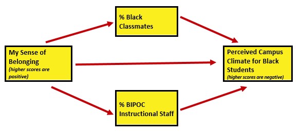
As I think about “how these variables go together” (which is often where I start in planning a study), I suspect parallel mediation. That is the perception of campus climate for Black students would be predicted by the respondent’s sense of belonging, mediated in separate paths through the proportion of classmates who are Black and the proportion of BIPOC instructional staff.
I would like to assess the model by having the instructional staff variable to be the %Black instructional staff. At the time that this lecture is being prepared, there is not sufficient Black representation in the instructional staff to model this.
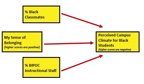
As in the data diagnostic chapter, I will conclude this chapter by conducting a statistical analysis with the multiply imputed data. Because parallel mediation can be complicated (I teach it in a later chapter), I will demonstrate use of our prepared variables with a simple multiple regression.
4.4 Multiple Imputation – a Super Brief Review
Multiple imputation is complex. Numerous quantitative psychologists had critiqued it and provided numerous cautions and guidelines for its use (Enders, 2010, 2017; R. J. A. Little & Rubin, 2002; T. D. Little et al., 2008). In brief,
4.4.1 Steps in Multiple Imputation
- Multiple imputation starts with a raw data file.
- Multiple imputation assumes that data are MAR (remember, MCAR is the more prestigious one). This means that researchers assume that missing values can be replaced by predictions derived from the observable portion of the dataset.
- Multiple imputation assumes that data are MAR (remember, MCAR is the more prestigious one). This means that researchers assume that missing values can be replaced by predictions derived from the observable portion of the dataset.
- Multiple datasets (often 5 to 20) are created where missing values are replaced via a randomized process (so the same missing value [item 4 for person A] will likely have different values for each dataset).
- The desired analysis is conducted simultaneously/separately for each of the imputed sets (so if you imputed 5 sets and wanted a linear regression, you get 5 linear regressions).
- A pooled analysis uses the point estimates and the standard errors to provide a single result that represents the analysis.
In a web-hosted guide from the University of Virginia Library, Katitas (2019) provided a user-friendly review and example of using tools in R in a multiple imputation. Katitas’ figure is a useful conceptual tool in understanding how multiple imputation works. This figure is my recreation of Katitas’ original.
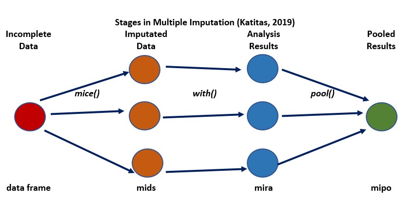
- the dataframe with missing data is the single place we start
- we intervene with a package like mice() to
- impute multiple sets of data (filling in the missing variables with different values that are a product of their conditional distribution and an element of “random”);
- “mids” (“multiply imputed dataset”) is an object class where the completed datasets are stored.
- the “with_mids” command allows OLS regression to be run, as many times as we have imputed datasets (in this figure, 3X). It produces different regression coefficients for each datset
- the “pool” command pools together the multiple coefficients taking into consideration the value of the coefficients,the standard errors, and the variance of the missing value parameter across the samples.
4.4.2 Statistical Approaches to Multiple Imputation
Joint multivariate normal distribution multiple imputation assumes that the observed data follow a multivariate normal distribution. The algorithm used draws from this assumed distribution. A drawback is that if the data do not follow a multivariate normal distribution, the imputed values are incorrect. Amelia and norm packages use this approach.
Conditional multiple imputation is an iterative procedure, modeling the conditional distribution of a certain variable given the other variables. In this way the distribution is assumed for each variable, rather than or the entire dataset. mice uses this approach.
mice: multivariate imputation by chained equations
4.5 Working the Problem
Katitas (2019) claims that it is best to impute the data in its rawest form possible because any change would be taking it away from its original distribution. There are debates about how many variables to include in an imputation. Some authors would suggest that researchers include everything that was collected. Others (like me) will trim the dataset to include (a) the variables included in the model, plus (b) auxiliary variables (i.e., variables not in the model, but that are sufficiently non-missing and will provide additional information to the data).
In our case we will want:
Item for the variables represented in our model
- the item level responses to the scales/subscales
- respondents’ sense of belonging to campus (3 items)
- respondents’ rating of campus climate for Black students (6 items)
- proportion of BIPOC instructional staff
- proportion of classmates who are Black
Auxiliary variables – let’s choose four. One will be the format of the course. Three items will be from the course evaluation.
- format, whether the course was taught in-person, a blend, or virtual
- cEval_1, “Course material was presented clearly”
- cEval_13, “Where applicable, issues were considered from multiple perspectives”
- cEval_19, “My understanding of the subject matter increased over the span of the course”
4.5.1 Selecting and Formatting Variables
There are some guidelines for selecting and formatting variables for imputation.
- Variables should be in their most natural state
- Redundant or too highly correlated variables should not be included
- If you reverse coded a variable (we haven’t yet), that’s ok, but if you have already reverse-coded, then exclude the original variable
- Redundant variables (or multicollinear variables) may cause the multiple imputation process to cease
- Violation of this also provides clues for troubleshooting
- Exclude variables with more than 25% missing
To make this as realistic as possible. Let’s start with our very raw data. The Scrubbing chapter provides greater detail on importing data directly from Qualtrics. If you have worked the lessons, consecutively, you know that data can be added to this survey at any time. So that the values in the chapter are consistent, I will use the datafiles that I immediately saved when I conducted the analysis at the time I last updated the chapter.
Please download the .rds or .csv file from MultivModel GitHub site. Please the file in the same folder as your .rmd file. As always, I prefer working with .rds files.
QTRX_df2 <- readRDS("QTRX_df230902b.rds")
# QTRX_df <- read.csv('QTRX_df230902b.csv', header = TRUE)
Next, I apply inclusion/exclusion criteria. As described in the Scrubbing chapter this includes:
- excluding all previews
- including only those who consented
- including only those whose rated course was offered by a U.S. institution
library(tidyverse)
QTRX_df2 <- dplyr::filter(QTRX_df2, DistributionChannel != "preview")
QTRX_df2 <- dplyr::filter(QTRX_df2, Consent == 1)
QTRX_df2 <- dplyr::filter(QTRX_df2, USinst == 0)
Preparing the data also meant renaming some variables that started with numbers (a hassle in R). I also renamed variables on the Campus Climate scale so that we know to which subscale they belong.
# renaming variables that started with numbers
QTRX_df2 <- dplyr::rename(QTRX_df2, iRace1 = "1_iRace", iRace2 = "2_iRace",
    iRace3 = "3_iRace", iRace4 = "4_iRace", iRace5 = "5_iRace", iRace6 = "6_iRace",
    iRace7 = "7_iRace", iRace8 = "8_iRace", iRace9 = "9_iRace", iRace10 = "10_iRace")
# renaming variables from the identification of classmates
QTRX_df2 <- dplyr::rename(QTRX_df2, cmBiMulti = Race_10, cmBlack = Race_1,
    cmNBPoC = Race_7, cmWhite = Race_8, cmUnsure = Race_2)
The Qualtrics download does not include an ID number. Because new variables are always appended to the end of the df, we also include code to make this the first column.
QTRX_df2 <- QTRX_df2 %>%
    dplyr::mutate(ID = row_number())
# moving the ID number to the first column; requires
QTRX_df2 <- QTRX_df2 %>%
    dplyr::select(ID, everything())
Because this huge df is cumbersome to work with, let’s downsize it to be closer to the size we will work with in the imputation
mimp_df <- dplyr::select(QTRX_df2, ID, iRace1, iRace2, iRace3, iRace4,
    iRace5, iRace6, iRace7, iRace8, iRace9, iRace10, cmBiMulti, cmBlack,
    cmNBPoC, cmWhite, cmUnsure, Belong_1:Belong_3, Blst_1:Blst_6, cEval_1,
    cEval_13, cEval_19, format)
# glimpse(mimp_df)
head(mimp_df)
# A tibble: 6 × 29
ID iRace1 iRace2 iRace3 iRace4 iRace5 iRace6 iRace7 iRace8 iRace9 iRace10
<int> <dbl> <dbl> <dbl> <dbl> <lgl> <lgl> <lgl> <lgl> <lgl> <lgl>
1 1 3 1 3 NA NA NA NA NA NA NA
2 2 3 NA NA NA NA NA NA NA NA NA
3 3 3 1 NA NA NA NA NA NA NA NA
4 4 3 1 3 NA NA NA NA NA NA NA
5 5 1 NA NA NA NA NA NA NA NA NA
6 6 3 NA NA NA NA NA NA NA NA NA
# ℹ 18 more variables: cmBiMulti <dbl>, cmBlack <dbl>, cmNBPoC <dbl>,
# cmWhite <dbl>, cmUnsure <dbl>, Belong_1 <dbl>, Belong_2 <dbl>,
# Belong_3 <dbl>, Blst_1 <dbl>, Blst_2 <dbl>, Blst_3 <dbl>, Blst_4 <dbl>,
# Blst_5 <dbl>, Blst_6 <dbl>, cEval_1 <dbl>, cEval_13 <dbl>, cEval_19 <dbl>,
# format <dbl>4.5.2 Creating Composite Variables
Qualtrics imports many of the categorical variables as numbers. R often reads them numerically (integers or numbers). If they are directly converted to factors, R will sometimes collapse. In this example, if there is a race that is not represented (e.g., 2 for BiMulti), when the numbers are changed to factors, R will assume it’s ordered and will change up the numbers. Therefore, it is ESSENTIAL to check (again and again ad nauseum) to ensure that your variables are recoding in a manner you understand.
mimp_df$iRace1 = factor(mimp_df$iRace1, levels = c(0, 1, 2, 3, 4), labels = c("Black",
    "nBpoc", "BiMulti", "White", "NotNotice"))
mimp_df$iRace2 = factor(mimp_df$iRace2, levels = c(0, 1, 2, 3, 4), labels = c("Black",
    "nBpoc", "BiMulti", "White", "NotNotice"))
mimp_df$iRace3 = factor(mimp_df$iRace3, levels = c(0, 1, 2, 3, 4), labels = c("Black",
    "nBpoc", "BiMulti", "White", "NotNotice"))
mimp_df$iRace4 = factor(mimp_df$iRace4, levels = c(0, 1, 2, 3, 4), labels = c("Black",
    "nBpoc", "BiMulti", "White", "NotNotice"))
mimp_df$iRace5 = factor(mimp_df$iRace5, levels = c(0, 1, 2, 3, 4), labels = c("Black",
    "nBpoc", "BiMulti", "White", "NotNotice"))
mimp_df$iRace6 = factor(mimp_df$iRace6, levels = c(0, 1, 2, 3, 4), labels = c("Black",
    "nBpoc", "BiMulti", "White", "NotNotice"))
mimp_df$iRace7 = factor(mimp_df$iRace7, levels = c(0, 1, 2, 3, 4), labels = c("Black",
    "nBpoc", "BiMulti", "White", "NotNotice"))
mimp_df$iRace8 = factor(mimp_df$iRace8, levels = c(0, 1, 2, 3, 4), labels = c("Black",
    "nBpoc", "BiMulti", "White", "NotNotice"))
mimp_df$iRace9 = factor(mimp_df$iRace9, levels = c(0, 1, 2, 3, 4), labels = c("Black",
    "nBpoc", "BiMulti", "White", "NotNotice"))
mimp_df$iRace10 = factor(mimp_df$iRace10, levels = c(0, 1, 2, 3, 4), labels = c("Black",
"nBpoc", "BiMulti", "White", "NotNotice"))This is a quick recap of how we calculated the proportion of instructional staff who are BIPOC.
# creating a count of BIPOC faculty identified by each respondent
mimp_df$count.BIPOC <- apply(mimp_df[c("iRace1", "iRace2", "iRace3", "iRace4",
    "iRace5", "iRace6", "iRace7", "iRace8", "iRace9", "iRace10")], 1, function(x) sum(x %in%
    c("Black", "nBpoc", "BiMulti")))

# creating a count of all instructional faculty identified by each
# respondent
mimp_df$count.nMiss <- apply(mimp_df[c("iRace1", "iRace2", "iRace3", "iRace4",
    "iRace5", "iRace6", "iRace7", "iRace8", "iRace9", "iRace10")], 1, function(x) sum(!is.na(x)))

# calculating the proportion of BIPOC faculty with the counts above
mimp_df$iBIPOC_pr = mimp_df$count.BIPOC/mimp_df$count.nMiss
I have included another variable, format that we will use as auxiliary variable. As written, these are the following meanings:
- In-person (all persons are attending in person)
- In person (some students are attending remotely)
- Blended: some sessions in person and some sessions online/virtual
- Online or virtual
- Other
Let’s recoded it to have three categories:
- 100% in-person (1)
- Some sort of blend/mix (2, 3)
- 100% online/virtual (4) NA. Other (5)
# we can assign more than one value to the same factor by repeating
# the label
mimp_df$format = factor(mimp_df$format, levels = c(1, 2, 3, 4, 5), labels = c("InPerson",
    "Blend", "Blend", "Online", is.na(5)))
Let’s trim the df again to just include the variables we need in the imputation.
mimp_df <- select(mimp_df, ID, iBIPOC_pr, cmBlack, Belong_1:Belong_3, Blst_1:Blst_6,
    cEval_1, cEval_13, cEval_19, format)
Recall one of the guidelines was to remove variables with more than 25% missing. This code calculates the proportion missing from our variables and places them in rank order.
p_missing <- unlist(lapply(mimp_df, function(x) sum(is.na(x))))/nrow(mimp_df)
sort(p_missing[p_missing > 0], decreasing = TRUE)
Blst_1 Blst_4 Blst_3 Blst_5 Blst_6 Belong_1 Belong_3
0.13043478 0.10144928 0.08695652 0.08695652 0.08695652 0.07246377 0.07246377
Blst_2 Belong_2 cEval_1 cEval_19 iBIPOC_pr cmBlack cEval_13
0.07246377 0.05797101 0.05797101 0.05797101 0.04347826 0.04347826 0.04347826 Luckily, none of our variables have more than 25% missing. If we did have a variable with more than 25% missing, we would have to consider what to do about it.
Later we learn that we should eliminate case with greater than 50% missingness. Let’s write code for that, now.
#Calculating number and proportion of item-level missingness
mimp_df$nmiss <- mimp_df%>%
    dplyr::select(iBIPOC_pr:format) %>% #the colon allows us to include all variables between the two listed (the variables need to be in order)
    is.na %>%
    rowSums

mimp_df<- mimp_df%>%
  dplyr::mutate(prop_miss = (nmiss/15)*100) #11 is the number of variables included in calculating the proportion

mimp_df <- dplyr::filter(mimp_df, prop_miss <= 50)  #update df to have only those with at least 50% of complete data
Once again, trim the df to include only the data to be included in the imputation
4.5.3 The Multiple Imputation
Because multiple imputation is a random process, if we all want the same answers we need to set a random seed.
The program we will use is mice. mice assumes that each variable has a distribution and it imputes missing variables according to that distribution.
This means we need to correctly specify each variable’s format/role. mice will automatically choose a distribution (think “format”) for each variable; we can override this by changing the methods’ characteristics.
The following code sets up the structure for the imputation. I’m not an expert at this – just following the Katitas example.
library(mice)
# runs the mice code with 0 iterations
imp <- mice(mimp_df, maxit = 0)
# Extract predictor Matrix and methods of imputation
predM = imp$predictorMatrix
meth = imp$method
Here we code what format/role each variable should be.
# These variables are left in the dataset, but setting them = 0 means
# they are not used as predictors.  We want our ID to be retained in
# the df.  There's nothing missing from it, and we don't want it used
# as a predictor, so it will just hang out.
predM[, c("ID")] = 0

# If you like, view the first few rows of the predictor matrix
# head(predM)

# We don't have any ordered categorical variables, but if we did we
# would follow this format poly <- c('Var1', 'Var2')

# We don't have any dichotomous variables, but if we did we would
# follow this format log <- c('Var3', 'Var4')

# Unordered categorical variables (nominal variables), but if we did
# we would follow this format
poly2 <- c("format")

# Turn their methods matrix into the specified imputation models
# Remove the hashtag if you have any of these variables meth[poly] =
# 'polr' meth[log] = 'logreg'
meth[poly2] = "polyreg"

meth
ID iBIPOC_pr cmBlack Belong_1 Belong_2 Belong_3 Blst_1 Blst_2
"" "pmm" "" "pmm" "" "pmm" "pmm" "pmm"
Blst_3 Blst_4 Blst_5 Blst_6 cEval_1 cEval_13 cEval_19 format
"pmm" "pmm" "pmm" "pmm" "pmm" "" "pmm" "polyreg" This list (meth) contains all our variables; “pmm” is the default and is the “predictive mean matching” process used. We see that format (an unordered categorical variable) is noted as “polyreg.” If we had used other categorical variables (ordered/poly, dichotomous/log), we would have seen those designations, instead. If there is “” underneath it means the data is complete.
Our variables of interest are now configured to be imputed with the imputation method we specified. Empty cells in the method matrix mean that those variables aren’t going to be imputed.
If a variable has no missing values, it is automatically set to be empty. We can also manually set variables to not be imputed with the meth[variable]=““ command.
The code below begins the imputation process. We are asking for 5 datasets. If you have many cases and many variables, this can take awhile. How many imputations? Recommendations have ranged as low as five to several hundred.
# With this command, we tell mice to impute the mimp_df data, create
# 5 datasets, use predM as the predictor matrix and don't print the
# imputation process.  If you would like to see the process (or if
# the process is failing to execute) set print as TRUE; seeing where
# the execution halts can point to problematic variables (more notes
# at end of lecture)

imp2 <- mice(mimp_df, maxit = 5, predictorMatrix = predM, method = meth,
    print = FALSE)
We need to create a “long file” that stacks all the imputed data. Looking at the df in R Studio shows us that when imp = 0 (the pe-imputed data), there is still missingness. As we scroll through the remaining imputations, there are no NA cells.
# First, turn the datasets into long format This procedure is, best I
# can tell, unique to mice and wouldn't work for repeated measures
# designs
mimp_long <- mice::complete(imp2, action = "long", include = TRUE)
If we look at it, we can see 6 sets of data. If the ID variable is sorted we see that:
- .imp = 0 is the unimputed set; there are still missing values
- .imp = 1, 2, 3, or 5 has no missing values for the variables we included in the imputation
With the code below we can see the proportion of missingness for each variable (that has missing data), sorted from highest to lowest.
p_missing_mimp_long <- unlist(lapply(mimp_long, function(x) sum(is.na(x))))/nrow(mimp_long)
sort(p_missing_mimp_long[p_missing_mimp_long > 0], decreasing = TRUE)  #check to see if this works
Blst_1 Blst_4 iBIPOC_pr Blst_3 Blst_5 Blst_6
0.012820513 0.007692308 0.005128205 0.005128205 0.005128205 0.005128205
Belong_1 Belong_3 Blst_2 cEval_1 cEval_19
0.002564103 0.002564103 0.002564103 0.002564103 0.002564103 4.5.4 Creating Scale Scores
Because our imputation was item-level, we need to score the variables with scales/subscales. As demonstrated more completely in the Scoring chapter, this required reversing one item in the campus climate scale:
mimp_long <- mimp_long %>%
    mutate(rBlst_1 = 8 - Blst_1)  #if you had multiple items, you could add a pipe (%>%) at the end of the line and add more until the last one
Below is the scoring protocol we used in the AIA protocol for scoring. Although the protocol below functionally says, “Create a mean score if (65-80)% is non-missing, for the imputed version, it doesn’t harm anything to leave this because there is no missing data.
# Making the list of variables
Belonging_vars <- c("Belong_1", "Belong_2", "Belong_3")
ResponseBL_vars <- c("rBlst_1", "Blst_4", "Blst_6")
StigmaBL_vars <- c("Blst_2", "Blst_3", "Blst_5")
ClimateBL_vars <- c("rBlst_1", "Blst_4", "Blst_6", "Blst_2", "Blst_3",
    "Blst_5")

# Creating the new variables
mimp_long$Belonging <- sjstats::mean_n(mimp_long[, Belonging_vars], 0.65)
mimp_long$ResponseBL <- sjstats::mean_n(mimp_long[, ResponseBL_vars], 0.8)
mimp_long$StigmaBL <- sjstats::mean_n(mimp_long[, StigmaBL_vars], 0.8)
mimp_long$ClimateBL <- sjstats::mean_n(mimp_long[, ClimateBL_vars], 0.8)
4.6 Multiple Regression with Multiply Imputed Data
For a refresher, here was the script when we used the AIA approach for managing missingness:
Climate_fit <- lm(ClimateBL ~ Belonging + cmBlack + iBIPOC_pr, data = item_scores_df)
summary(Climate_fit)
In order for the regression to use multiply imputed data, it must be a “mids” (multiply imputed data sets) type
Here’s what we do with imputed data:
In this process, 5 individual, OLS, regressions are being conducted and the results being pooled into this single set.
# A tibble: 20 × 6
   term        estimate std.error statistic       p.value  nobs
   <chr>          <dbl>     <dbl>     <dbl>         <dbl> <int>
 1 (Intercept)   3.02      0.435      6.95  0.00000000283    65
 2 Belonging    -0.0311    0.0897    -0.346 0.730            65
 3 cmBlack      -0.0206    0.0165    -1.25  0.215            65
 4 iBIPOC_pr    -0.663     0.339     -1.95  0.0552           65
 5 (Intercept)   3.02      0.446      6.77  0.00000000578    65
 6 Belonging    -0.0349    0.0907    -0.385 0.702            65
 7 cmBlack      -0.0234    0.0166    -1.41  0.165            65
 8 iBIPOC_pr    -0.470     0.329     -1.43  0.158            65
 9 (Intercept)   3.01      0.450      6.70  0.00000000744    65
10 Belonging    -0.0349    0.0915    -0.381 0.704            65
11 cmBlack      -0.0222    0.0167    -1.33  0.187            65
12 iBIPOC_pr    -0.485     0.330     -1.47  0.147            65
13 (Intercept)   2.95      0.448      6.57  0.0000000127     65
14 Belonging    -0.0152    0.0920    -0.165 0.870            65
15 cmBlack      -0.0216    0.0168    -1.29  0.203            65
16 iBIPOC_pr    -0.558     0.343     -1.62  0.110            65
17 (Intercept)   3.00      0.452      6.64  0.00000000963    65
18 Belonging    -0.0311    0.0921    -0.337 0.737            65
19 cmBlack      -0.0214    0.0168    -1.28  0.207            65
20 iBIPOC_pr -0.531 0.337 -1.57 0.121 65Class: mipo m = 5
term m estimate ubar b t dfcom
1 (Intercept) 5 2.99980658 0.1990231323 0.000999315858 0.2002223113 61
2 Belonging 5 -0.02940746 0.0083160161 0.000067017541 0.0083964371 61
3 cmBlack 5 -0.02184241 0.0002777582 0.000001056566 0.0002790261 61
4 iBIPOC_pr 5 -0.54138195 0.1128248694 0.005817914953 0.1198063673 61
df riv lambda fmi
1 58.70890 0.006025325 0.005989238 0.03820536
2 58.44929 0.009670622 0.009577997 0.04181342
3 58.80737 0.004564689 0.004543947 0.03675551
4 53.13966 0.061879070 0.058273179 0.09182261 term estimate std.error statistic df p.value
1 (Intercept) 2.99980658 0.44746208 6.7040465 58.70890 0.000000008735881
2 Belonging -0.02940746 0.09163207 -0.3209298 58.44929 0.749408305666738
3 cmBlack -0.02184241 0.01670407 -1.3076097 58.80737 0.196094825405891
4 iBIPOC_pr -0.54138195 0.34613056 -1.5640975 53.13966 0.123730969370680Results of a multiple regression predicting the respondents’ perceptions of campus climate for Black students indicated that neither contributions of the respondents’ personal belonging (\(B = -0.029, p = 0.749),the proportion of BIPOC instructional staff (\)B = -0.541, p = 0.124), nor proportion of Black classmates (\(B = -0.022, p = 0.196\)) led to statistically significant changes in perceptions of campus climate for Black students. Results are presented in Table X.
4.7 Toward the APA Style Write-up
4.7.1 Method/Data Diagnostics
Data screening suggested that 107 individuals opened the survey link. Of those, 83 granted consent and proceeded into the survey items. A further inclusion criteria was that the course was taught in the U.S; 69 met this criteria.
Across cases that were deemed eligible on the basis of the inclusion/exclusion criteria, missingness ranged from 0 to 67%. Across the dataset, 3.86% of cells had missing data and 87.88% of cases had nonmissing data. At this stage in the analysis, we allowed all cases with fewer than 50% missing to be included the multiple imputation (Katitas, 2019).
Regarding the distributional characteristics of the data, skew and kurtosis values of the variables fell below the values of 3 (skew) and 10 (kurtosis) that Kline suggests are concerning (2016b). Results of the Shapiro-Wilk test of normality indicate that our variables assessing the proportion of classmates who are Black (\(W = 0.878, p < 0.001\)) and the proportion of BIPOC instructional staff(\(W = 0.787, p < 0.001\)) are statistically significantly different than a normal distribution. The scales assessing the respondent’s belonging (\(0.973, p = 0.165\)) and the respondent’s perception of campus climate for Black students (\(W = 0.951, p = 0.016\)) did not differ differently from a normal distribution.
We evaluated multivariate normality with the Mahalanobis distance test. Specifically, we used the psych::outlier() function and included all continuous variables in the calculation. Our visual inspection of the Q-Q plot suggested that the plotted line strayed from the straight line as the quantiles increased. Additionally, we appended the Mahalanobis distance scores as a variable to the data. Analyzing this variable, we found that 1 case exceed three standard deviations beyond the median. Given that the Mahalanobis distance values increased in a consistent manner (i.e., no extreme “jumps”) we retained all cases.
We managed missing data with multiple imputation (Enders, 2017; Katitas, 2019). We imputed five sets of data with the R package, mice (v. 3.13) – a program that utilizes conditional multiple imputation. The imputation included the item-level variables that comprised our scales, the variables that represented proportion of BIPOC instructional staff and proportion of Black classmates, as well as four auxiliary variables (three variables from the course evaluation and the format [in-person/blended/virtual] of the class).
4.7.2 Results
Results of a multiple regression predicting the respondents’ perceptions of campus climate for Black students indicated that neither contributions of the respondents’ personal belonging (\(B = -0.029, p = 0.749), the proportion of BIPOC instructional staff (\)B = -0.541, p = 0.124), nor proportion of Black classmates (\(B = -0.022, p = 0.196\)) led to statistically significant changes in perceptions of campus climate for Black students. Results are presented in Table X.
Some notes about this write-up
- I went ahead and used the data diagnostics that we did in the AIA method. It feels to me like these should be calculated with the multiply imputed data (i.e., 5 sets, with pooled estimates and standard errors), but I do not see that modeled – anywhere in R.
- Note the similarities with the AIA write-up.
4.8 Multiple imputation considerations
- Character vectors (i.e., values that are represented with words) can be problematic. If they are causing trouble, consider
- recode into factors,
- keep it in the df, but exclude it from the imputation protocol,
- our “format” variable was an ordered factor (i.e., each term was associated with a value), so I think that helped us avoid problems
- Variables with really high (like 50% or more) proportions of missingness should be excluded.
- Variables that are highly correlated or redundant (even if inverse) will halt the execution. If you set print=TRUE you will see where the algorithm is having difficulty because it will halt at that variable.
- Variables with non-missing values can be problematic. If they are problematic, just exclude them from the process.
*Width (columns/variables) versus length (rows/cases). You must have more rows/cases than columns/variables. It is difficult to say how many. If this is a problem:
- Consider scoring scales first with AIA, then impute with whole scales.
- Divide the df in halves or thirds, impute separately, then join with the ID numbers.
- There should be auxiliary variables in each. *Item-level imputation is its “whole big thing” with multiple, complex considerations. There are tremendous resources
- Enders BLIMP app is free and works with R
- Little’s (2002) article
- How many imputations? Controversial and has changed over the years.
- Practical concern: the more you request, the longer it will take in R, this demo was 5
- For a number of years there was a push for 20, but I’ve also seen recommendations for 100s.
- Check examples of imputed studies in your disciplinary specialty/journals.
- There are lots of discussions and debates about
- allowing for fractional/decimal responses (a 3.5 on 1 to 4 scaling; or a 0.75 on a dichotomous variable such as male/female)
- out-of-bounds estimates (what if you get a 7 on 1 to 4 scaling?)
4.9 Practice Problems
The three problems described below are designed to be continuations from the previous chapters. You will likely encounter challenges that were not covered in this chapter. Search for and try out solutions, knowing that there are multiple paths through the analysis. In addition to the scrubbing, scoring, and data diagnostic skills learned in the prior lessons, the overall notion of the suggestions for practice are to (a) multiply impute a minimum of 5 sets of data, (b) repeat the regression (attempted in the Data Dx chapter), (c) create APA style write-ups of the multiple imputation method and regression results, and (d) explain it to someone.
4.9.1 Problem #1: Reworking the Chapter Problem
If you chose this option in the prior chapters, you imported the data from Qualtrics, applied inclusion/exclusion criteria, renamed variables, downsized the df to the variables of interest, properly formatted the variables, interpreted item-level missingness, scored the scales/subscales, interpreted scale-level missingness, and wrote up the results. Please continue with the remaining tasks.
4.9.2 Problem #2: Use the Rate-a-Recent-Course Survey, Choosing Different Variables
If you chose this option in the prior chapter, you chose a minimum of three variables from the Rate-a-Recent-Course survey to include in a simple statistical model. You imported the data from Qualtrics, applied inclusion/exclusion criteria, renamed variables, downsized the df to the variables of interest, properly formatted the variables, interpreted item-level missingness, scored the scales/subscales, interpreted scale-level missingness, and wrote up the results. Please continue with the remaining tasks.
4.9.3 Problem #3: Other data
If you chose this option in the prior chapter, you used raw data that was available to you. You imported it into R, applied inclusion/exclusion criteria, renamed variables, downsized the df to the variables of interest, properly formatted the variables, interpreted item-level missingness, scored the scales/subscales, interpreted scale-level missingness, and wrote up the results. Please continue with the remaining tasks.
4.9.4 Grading Rubric
| Assignment Component | Points Possible | Points Earned |
|---|---|---|
| 1. Specify a research model with three predictor variables (continuously or categorically scaled) and one dependent (continuously scaled) variable. | 5 | _____ |
| 2. Import the raw data | 5 | _____ |
| 3. Apply inclusionary/exclusionary criteria | 5 | _____ |
| 4. Format any variables that shouldn’t be imputed in their raw form | 5 | _____ |
| 5. Multiply impute a minimum of 5 sets of data | 5 | _____ |
| 6. Run a regression (for multiply imputed data) with at least three variables | 5 | _____ |
| 7. APA style write-up of the multiple imputation section of data diagnostics | 5 | _____ |
| 8. APA style write-up regression results | 5 | _____ |
| 9. Explanation to grader | 5 | _____ |
| Totals | 45 | _____ |
4.10 Homeworked Example
For more information about the data used in this homeworked example, please refer to the description and codebook located at the end of the introductory lesson in ReCentering Psych Stats. An .rds file which holds the data is located in the Worked Examples folder at the GitHub site the hosts the OER. The file name is ReC.rds.
Although the lessons focused on preparing data for analyses were presented in smaller sections, this homeworked example combines the suggestions for practice from the Scrubbing, Scoring, Data Dx because they are also used when missing data is managed with multiple imputation. My hope is that is cumulative presentation is a closer approximation of what researchers need for their research projects.
These lessons were created to prepare a set of data to analyze a specific research model. Consequently, the model should be known and described at the beginning.
4.10.1 Scrubbing
Specify a research model
A further assignment requirement was that the model should include three predictor variables (continuously or categorically scaled) and one dependent (continuously scaled) variable.
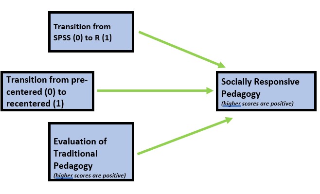
As in the homeworked example for the Data Dx lesson, I am hypothesizing that socially responsive pedagogy (my dependent variable) will increase as a function of:
- the transition from SPSS (0) to R(1),
- the transition from a pre-centered (0) to re-centered (1) curriculum, and
- higher evaluations of traditional pedagogy
Because this data is nested within the person (i.e., students can contribute up to three course evaluations over the ANOVA, multivariate, and psychometrics courses) proper analysis would require a statistic (e.g., multilevel modeling) that would address the dependency in the data. Therefore, I will include only those students who are taking the multivariate modeling class.
While it is possible to conduct multiple imputation at the scale level, we will do so at the item-level (i.e., before we compute the scale scores).
If you wanted to use this example and dataset as a basis for a homework assignment, you could create a different subset of data. I worked the example for students taking the multivariate modeling class. You could choose ANOVA or psychometrics. You could also choose a different combinations of variables.
Apply inclusionary/exclusionary criteria
Because this data is publicly posted on the Open Science Framework, it was necessary for me to already exclude those individuals. This data was unique in that students could freely write some version of “Opt out.” My original code included a handful of versions, but here was the basic form:
# testing to see if my code worked raw <- dplyr::filter (raw,
# SPFC.Decolonize.Opt.Out != 'Okay')
raw <- dplyr::filter(raw, SPFC.Decolonize.Opt.Out != "Opt Out")
I want to exclude students’ responses for the ANOVA and psychometrics courses.
At this point, these my only inclusion/exclusion criteria. I can determine how many students (who consented) completed any portion of the survey.
[1] 844.10.1.1 Format any variables that shouldn’t be imputed in their raw form
Let’s first create a df with the item-level variables that will fuel our model.
In addition to the variables in our model, we will include four auxiliary variables. These include Dept (Department: Clinical or Industrial-Organizational) and four additional course evaluation items: OvInstructor, MyContribution, IncrInterest, IncrUnderstanding.
Let’s check the structure to be certain that StatsPkg (SPSS, R) and Centered (Pre, Re) are ordered factors. We also want the course evaluation items to be integer (or numerical).
mimp_df <- dplyr::select(raw, deID, StatsPkg, Centering, ClearResponsibilities,
    EffectiveAnswers, Feedback, ClearOrganization, ClearPresentation, InclusvClassrm,
    EquitableEval, MultPerspectives, DEIintegration, Dept, OvInstructor,
    MyContribution, IncrInterest, IncrUnderstanding)
str(mimp_df)
Classes 'data.table' and 'data.frame': 84 obs. of 17 variables:
$ deID : int 11 12 13 14 15 16 17 18 35 19 ...
$ StatsPkg : Factor w/ 2 levels "SPSS","R": 2 2 2 2 2 2 2 2 2 2 ...
$ Centering : Factor w/ 2 levels "Pre","Re": 2 2 2 2 2 2 2 2 2 2 ...
$ ClearResponsibilities: int 4 5 5 5 4 3 5 5 3 5 ...
$ EffectiveAnswers : int 4 5 5 4 4 3 5 5 4 4 ...
$ Feedback : int 4 5 4 4 5 4 5 4 4 5 ...
$ ClearOrganization : int 3 5 5 4 4 3 5 5 4 5 ...
$ ClearPresentation : int 4 5 5 3 4 2 5 4 5 5 ...
$ InclusvClassrm : int 5 5 5 5 5 4 5 5 5 5 ...
$ EquitableEval : int 4 5 5 5 4 4 5 4 5 5 ...
$ MultPerspectives : int 4 5 5 5 5 5 5 4 5 5 ...
$ DEIintegration : int 5 5 5 5 5 5 5 5 5 5 ...
$ Dept : chr "CPY" "CPY" "CPY" "CPY" ...
$ OvInstructor : int 3 5 5 3 5 2 5 4 5 5 ...
$ MyContribution : int 4 5 4 3 4 3 5 4 4 5 ...
$ IncrInterest : int 4 5 4 3 4 3 5 4 5 4 ...
$ IncrUnderstanding : int 4 5 5 3 4 3 5 4 5 5 ...
- attr(*, ".internal.selfref")=<externalptr> Factor w/ 2 levels "CPY","ORG": 1 1 1 1 1 1 1 1 1 1 ...We should eliminate case with greater than 50% missingness.
library(tidyverse)
#Calculating number and proportion of item-level missingness
mimp_df$nmiss <- mimp_df%>%
    dplyr::select(StatsPkg:IncrUnderstanding) %>% #the colon allows us to include all variables between the two listed (the variables need to be in order)
    is.na %>%
    rowSums

mimp_df<- mimp_df%>%
  dplyr::mutate(prop_miss = (nmiss/13)*100) #11 is the number of variables included in calculating the proportion

mimp_df <- filter(mimp_df, prop_miss <= 50)  #update df to have only those with at least 50% of complete data
Once again, trim the df to include only the data to be included in the imputation
4.10.1.2 Multiply impute a minimum of 5 sets of data
Because multiple imputation is a random process, if we all want the same answers we need to set a random seed.
The program we will use is mice. mice assumes that each variable has a distribution and it imputes missing variables according to that distribution.
This means we need to correctly specify each variable’s format/role. mice will automatically choose a distribution (think “format”) for each variable; we can override this by changing the methods’ characteristics.
The following code sets up the structure for the imputation. This follows the Katitas example.
library(mice)
# runs the mice code with 0 iterations
imp <- mice(mimp_df, maxit = 0)
# Extract predictor Matrix and methods of imputation
predM = imp$predictorMatrix
meth = imp$method
log = imp$log
Here we code what format/role each variable should be.
# These variables are left in the dataset, but setting them = 0 means
# they are not used as predictors.  We want our ID to be retained in
# the df.  There's nothing missing from it, and we don't want it used
# as a predictor, so it will just hang out.
predM[, c("deID")] = 0

# If you like, view the first few rows of the predictor matrix
# head(predM)

# We don't have any ordered categorical variables, but if we did we
# would follow this format poly <- c('Var1', 'Var2')

# We have three dichotomous variables
log <- c("StatsPkg", "Centering", "Dept")

# Unordered categorical variables (nominal variables), but if we did
# we would follow this format poly2 <- c('format')

# Turn their methods matrix into the specified imputation models
# Remove the hashtag if you have any of these variables meth[poly] =
# 'polr'
meth[log] = "logreg"
# meth[poly2] = 'polyreg'

meth
deID StatsPkg Centering
"" "logreg" "logreg"
ClearResponsibilities EffectiveAnswers Feedback
"pmm" "" "pmm"
ClearOrganization ClearPresentation InclusvClassrm
"" "" "pmm"
EquitableEval MultPerspectives DEIintegration
"" "pmm" "pmm"
Dept OvInstructor MyContribution
"logreg" "" ""
IncrInterest IncrUnderstanding
"pmm" "" This list (meth) contains all our variables; “pmm” is the default and is the “predictive mean matching” process used. We see that StatsPkg and Centering are noted as “logreg.” This is because they are dichotomous variables. If there is ““ underneath it means the data is complete. The data will be used in imputing other data, but none of that data will be imputed.
Our variables of interest are now configured to be imputed with the imputation method we specified. Empty cells in the method matrix mean that those variables aren’t going to be imputed.
If a variable has no missing values, it is automatically set to be empty. We can also manually set variables to not be imputed with the meth[variable]=““ command.
The code below begins the imputation process. We are asking for 5 datasets. If you have many cases and many variables, this can take awhile. How many imputations? Recommendations have ranged as low as five to several hundred.
# With this command, we tell mice to impute the anesimpor2 data,
# create 5vvdatasets, use predM as the predictor matrix and don't
# print the imputation process.  If you would like to see the process
# (or if the process is failing to execute) set print as TRUE; seeing
# where the execution halts can point to problematic variables (more
# notes at end of lecture)

imp2 <- mice(mimp_df, maxit = 5, predictorMatrix = predM, method = meth,
    log = log, print = FALSE)
We need to create a “long file” that stacks all the imputed data. Looking at the df in R Studio shows us that when imp = 0 (the pe-imputed data), there is still missingness. As we scroll through the remaining imputations, there are no NA cells.
# First, turn the datasets into long format This procedure is, best I
# can tell, unique to mice and wouldn't work for repeated measures
# designs
mimp_long <- mice::complete(imp2, action = "long", include = TRUE)
If we look at it, we can see 6 sets of data. If the deID variable is sorted we see that:
- .imp = 0 is the unimputed set; there are still missing values
- .imp = 1, 2, 3, or 5 has no missing values for the variables we included in the imputation
With the code below we can see the proportion of missingness for each variable (that has missing data), sorted from highest to lowest.
p_missing_mimp_long <- unlist(lapply(mimp_long, function(x) sum(is.na(x))))/nrow(mimp_long)
sort(p_missing_mimp_long[p_missing_mimp_long > 0], decreasing = TRUE)  #check to see if this works
DEIintegration InclusvClassrm Feedback
0.027777778 0.007936508 0.003968254
ClearResponsibilities MultPerspectives IncrInterest
0.001984127 0.001984127 0.001984127 Because our imputation was item-level, we need to score the variables with scales/subscales.
Traditional pedagogy is a predictor variable that needs to be created by calculating the mean if at least 75% of the items are non-missing. None of the items need to be reverse-scored. I will return to working with the scrub_df data.
# this seems to work when I build the book, but not in 'working the
# problem'
TradPed_vars <- c("ClearResponsibilities", "EffectiveAnswers", "Feedback",
    "ClearOrganization", "ClearPresentation")
# mimp_long$TradPed <- sjstats::mean_n(mimp_long[, TradPed_vars],
# .75)

# this seems to work when I 'work the problem' (but not when I build
# the book) the difference is the two dots before the last SRPed_vars
mimp_long$TradPed <- sjstats::mean_n(mimp_long[, TradPed_vars], 0.75)
The dependent variable is socially responsive pedagogy. It needs to be created by calculating the mean if at least 75% of the items are non-missing. None of the items need to be reverse-scored.
# this seems to work when I build the book, but not in 'working the
# problem' SRPed_vars <- c('InclusvClassrm','EquitableEval',
# 'MultPerspectives', 'DEIintegration') mimp_long$SRPed <-
# sjstats::mean_n(mimp_long[, SRPed_vars], .75)

# this seems to work when I 'work the problem' (but not when I build
# the book) the difference is the two dots before the last SRPed_vars
SRPed_vars <- c("InclusvClassrm", "EquitableEval", "MultPerspectives",
    "DEIintegration")
mimp_long$SRPed <- sjstats::mean_n(mimp_long[, SRPed_vars], 0.75)
4.10.1.3 Run a regression (for multiply imputed data) with at least three variables
For comparison, here was the script when we used the AIA approach for managing missingness:
SRPed_fit <- lm(SRPed ~ StatsPkg + Centering + TradPed, data = scored)
In order for the regression to use multiply imputed data, it must be a “mids” (multiply imputed data sets) type
Here’s what we do with imputed data:
In this process, 5 individual, OLS, regressions are being conducted and the results being pooled into this single set.
# A tibble: 20 × 6
   term        estimate std.error statistic  p.value  nobs
   <chr>          <dbl>     <dbl>     <dbl>    <dbl> <int>
 1 (Intercept)    1.90     0.310      6.13  3.13e- 8    84
 2 StatsPkgR      0.187    0.118      1.59  1.16e- 1    84
 3 CenteringRe    0.117    0.108      1.09  2.79e- 1    84
 4 TradPed        0.565    0.0659     8.56  6.30e-13    84
 5 (Intercept)    1.94     0.314      6.17  2.62e- 8    84
 6 StatsPkgR      0.191    0.119      1.60  1.13e- 1    84
 7 CenteringRe    0.110    0.109      1.01  3.17e- 1    84
 8 TradPed        0.557    0.0667     8.36  1.63e-12    84
 9 (Intercept)    1.96     0.313      6.26  1.80e- 8    84
10 StatsPkgR      0.178    0.119      1.50  1.38e- 1    84
11 CenteringRe    0.111    0.109      1.02  3.10e- 1    84
12 TradPed        0.555    0.0665     8.35  1.69e-12    84
13 (Intercept)    2.03     0.325      6.24  1.98e- 8    84
14 StatsPkgR      0.185    0.123      1.50  1.38e- 1    84
15 CenteringRe    0.104    0.113      0.918 3.62e- 1    84
16 TradPed        0.539    0.0691     7.80  1.95e-11    84
17 (Intercept)    1.91     0.306      6.26  1.77e- 8    84
18 StatsPkgR      0.158    0.116      1.36  1.78e- 1    84
19 CenteringRe    0.117    0.107      1.10  2.76e- 1    84
20 TradPed 0.567 0.0649 8.73 2.93e-13 84 term estimate std.error statistic df p.value
1 (Intercept) 1.9480744 0.31833535 6.119567 74.55114 0.000000040039269753
2 StatsPkgR 0.1798400 0.11996611 1.499090 76.64577 0.137957984459613908
3 CenteringRe 0.1117906 0.10918108 1.023901 77.81162 0.309054914517060075
4 TradPed 0.5564494 0.06768356 8.221338 74.26455 0.000000000004825124Results of a multiple regression predicting the socially responsive course evaluation ratings indicated that neither the transition from SPSS to R (\(B = 0.178, p = 0.135\)) nor the transition to an explicitly recentered curriculum (\(B = 0.116, p = 0.285) led to statistically significant diferences. In contrast, traditional pedagogy had a strong, positive effect on evaluations of socially responsive pedagogy (\)B = 0.571, p < 0.001). Results of the regression model are presented in Table 2.
4.10.1.4 APA style write-up of the multiple imputation section of data diagnostics
My write-up draws from some of the results we obtained in the homeworked example at the end of the Data Dx chapter.
This is a secondary analysis of data involved in a more comprehensive dataset that included students taking multiple statistics courses (N = 310). Having retrieved this data from a repository in the Open Science Framework, only those who consented to participation in the study were included. Data used in these analyses were 84 students who completed the multivariate clas.
Across cases that were deemed eligible on the basis of the inclusion/exclusion criteria, missingness ranged from 0 to 100%. Across the dataset, 3.86% of cells had missing data and 87.88% of cases had nonmissing data. At this stage in the analysis, missingness for all cases did not exceed 50% (Katitas, 2019) and they were all included in the multiple imputation .
Regarding the distributional characteristics of the data, skew and kurtosis values of the variables fell below the values of 3 (skew) and 10 (kurtosis) that Kline suggests are concerning (2016b). Results of the Shapiro-Wilk test of normality indicate that our variables assessing the traditional pedagogy (\(W = 0.830, p < 0.001\)) and socially responsive pedagogy (0.818, p < 0.001) are statistically significantly different than a normal distribution. Inspection of distributions of the variables indicated that both course evaluation variables were negatively skewed, with a large proportion of high scores.
We evaluated multivariate normality with the Mahalanobis distance test. Specifically, we used the psych::outlier() function and included both continuous variables in the calculation. Our visual inspection of the Q-Q plot suggested that the plotted line strayed from the straight line as the quantiles increased. Additionally, we appended the Mahalanobis distance scores as a variable to the data. Analyzing this variable, we found that 2 cases exceed three standard deviations beyond the median.
We managed missing data with multiple imputation (Enders, 2017; Katitas, 2019). We imputed five sets of data with the R package, mice (v. 3.13) – a program that utilizes conditional multiple imputation. The imputation included the 9 item-level variables that comprised our scales and the dichotomous variable representing traditional pedagogy and socially responsive pedagogy. We also included five auxiliary variables (four variables from the course evaluation and the whether the student was from the Clinical or Industrial-Organizational Psychology program).
4.10.1.5 APA style write-up regression results
Results of a multiple regression predicting the socially responsive course evaluation ratings indicated that neither the transition from SPSS to R (\(B = 0.178, p = 0.135\)) nor the transition to an explicitly recentered curriculum (\(B = 0.116, p = 0.285) led to statistically significant diferences. In contrast, traditional pedagogy had a strong, positive effect on evaluations of socially responsive pedagogy (\)B = 0.571, p < 0.001). Results of the regression model are presented in Table 2.
As in the lesson itself, I used the data diagnostics that we did in the AIA method. It feels to me like these should be calculated with the multiply imputed data (i.e., 5 sets, with pooled estimates and standard errors), but I do not see that modeled – anywhere in tutorials I consulted.