Chapter 9 Establishing the Measurement Model
This lesson opens a series on structural equation modeling devoted to the full latent variable model. Full latent variable models test the directional linkages between variables in the model and they contain both (a) measurement and (b) structural components. Thus, evaluating a full latent variable model is completed in two larger steps which establish the measurement model first and then proceed to evaluating the structural model. The focus of this lesson is on the first step – establishing the measurement model.
9.2 Introduction to Structural Equation Modeling (SEM)
In the lesson progression in Recentering Psych Stats, we used ordinary least squares (OLS) approaches as we learned analysis of variance (and hopefully coming soon multiple regression). As we entered more complex modeling, we began to use maximum likelihood estimators (MLE). A comparison of these two approaches was provided in the lesson on Simple Moderation in OLS and MLE.
SEM is yet another progression in regression and it has several distinguishing aspects.
- SEM uses latent variables. Latent variables are not directly observed or measured (i.e., they do not exist as a column in your data). Rather, they are inferred from other observed variables. The latent variable (i.e., depression) is presumed to cause scores on the observed (sometimes termed manifest) variables. In these lessons, we can easily think of latent variables as the factor (or scale) and the observed/manifest variables as its items.
- To clarify, SEM models can incorporate latent (unobserved) and manifest (observed) in the same model.
- SEM evaluates causal processes through a series of structural (i.e., regression) equations.
- SEM provides global fit indices that provide an overall evaluation of the goodness of fit of the model. State another way, they indicate how closely the model’s predictions align with the actual data.
- SEM tests multiple hypotheses, simultaneously. That is, we can easily combine separate smaller models (e.g., simple mediation, simple moderation) into a grander model (e.g., moderated mediation).
- SEM permits multiple dependent variables. Actually, in SEM we typically refer to variables as exogenous (variables that only serve as predictors) and endogenous (variables that are predicted [even if they also predict]).
- In contrast to traditional multivariate procedures that can neither assess nor correct for measurement error, SEM provides explicit estimates of error variance parameters.
- SEM models have a long history of being represented pictorially and the conventions of these figures make it possible for them to efficiently convey the findings.
With all of these advantages, SEM is widely used for nonexperimental research.
In this lesson we start on the journey toward evaluating a full latent variable model; sometimes these are called hybrid models (SEM with Latent Variables (David A. Kenny), n.d.) because they are a mix of path analysis and confirmatory factor analysis (CFA). Today we focus on the CFA portion because we will specify (and likely respecify) the measurement model. In evaluating the measurement model we will specify a model where each of the constructs (factors) is represent in its latent form. That is each construct is represented as a factor (a latent variable) by its manifest, item-level, variables. In our measurement model we will allow all of the factors to covary with each other. It is important to note that this model will have the best fit of all because all of the structural paths are saturated. Stated another way, the subsequent test of the structural model will have worse fit. This means that if the fit of the measurement model is below our thresholds, we will investigate options for improving it before moving to evaluation of the structural model.
9.3 Workflow for Evaluating a Structural Model
The following workflow is one that provides an overview of the entire process of evaluating a structural model.
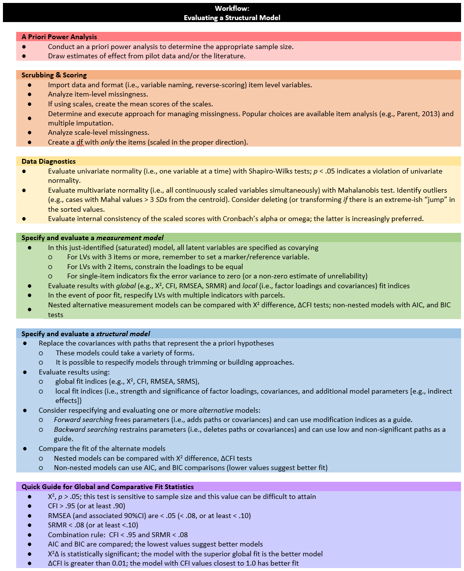 Evaluating a structural model involves the following steps:
- A Priori Power Analysis
- Conduct an a priori power analysis to determine the appropriate sample size. _ Draw estimates of effect from pilot data and/or the literature.
- Scrubbing & Scoring
- Import data and format (i.e., variable naming, reverse-scoring) item level variables.
- Analyze item-level missingness.
- If using scales, create the mean scores of the scales.
- Determine and execute approach for managing missingness. Popular choices are available item analysis (e.g., Parent, 2013) and multiple imputation.
- Analyze scale-level missingness.
- Create a df with only the items (scaled in the proper direction).
- Data Diagnostics
- Evaluate univariate normality (i.e., one variable at a time) with Shapiro-Wilks tests; p < .05 indicates a violation of univariate normality.
- Evaluate multivariate normality (i.e., all continuously scaled variables simultaneously) with Mahalanobis test. Identify outliers (e.g., cases with Mahal values > 3 SDs from the centroid). Consider deleting (or transforming if there is an extreme-ish “jump” in the sorted values.
- Evaluate internal consistency of the scaled scores with Cronbach’s alpha or omega; the latter is increasingly preferred. Specify and evaluate a measurement model
- In this just-identified (saturated) model, all latent variables are specified as covarying.
- For LVs with 3 items or more, remember to set a marker/reference variable,
- For LVs with 2 items, constrain the loadings to be equal,
- For single-item indicators fix the error variance to zero (or a non-zero estimate of unreliability).
- Evaluate results with global (e.g., X2, CFI, RMSEA, SRMR) and local (i.e., factor loadings and covariances) fit indices.
- In the event of poor fit, respecify LVs with multiple indicators with parcels.
- Nested alternative measurement models can be compared with Χ2 difference, ΔCFI tests; non-nested models with AIC, and BIC tests .
- Specify and evaluate a structural model.
- Replace the covariances with paths that represent the a priori hypotheses.
- These models could take a variety of forms.
- It is possible to respecify models through trimming or building approaches.
- Evaluate results using
- global fit indices (e.g., X2, CFI, RMSEA, SRMS),
- local fit indices (i.e., strength and significance of factor loadings, covariances, and additional model parameters [e.g., indirect effects]).
- Consider respecifying and evaluating one or more alternative models.
- Forward searching involves freeing parameters (adding paths or covariances) and can use modification indices as a guide.
- Backward searching involves restraining parameters (deleting paths or covariances) and can use low and non-significant paths as a guide.
- Compare the fit of the alternate models.
- Nested models can be compared with Χ2 difference and ΔCFI tests.
- Non-nested models can be compared with AIC and BIC (lower values suggest better fit).
- Replace the covariances with paths that represent the a priori hypotheses.
- Quick Guide for Global and Comparative Fit Statistics.
- \(\chi^2\), p < .05; this test is sensitive to sample size and this value can be difficult to attain
- CFI > .95 (or at least .90)
- RMSEA (and associated 90%CI) are < .05 ( < .08, or at least < .10)
- SRMR < .08 (or at least <.10)
- Combination rule: CFI < .95 and SRMR < .08
- AIC and BIC are compared; the lowest values suggest better models
- \(\chi^2\Delta\) is statistically significant; the model with the superior fit is the better model
- \(\delta CFI\) is greater than 0.01; the model with CFI values closest to 1.0 has better fit
The focus of this lesson in on the specification, evaluation, and respecification of the measurement model.
9.4 The Measurement Model: Specification and Evaluation
Structural models include both measurement and structural portions. The measurement model has two primary purposes. First the measurement model specifies the latent variables. That is, CFA-like models (i.e., one per latent variable) define each latent variable (i.e., scale score – but not “scored”) by its observed indicators (i.e., survey items). Resulting factor loadings indicate the strength of the relationships between the observed items and their latent variable.
Second, the measurement model allows the researchers to assess the goodness of model fit. A well-fitting model is required for accurately interpreting the relationships between the latent variables in the structural model. Additionally, the fit of the structural model will never surpass that of the measurement model. Stated another way – if the fit of the measurement model is inferior, the structural model is likely to be worse. There is at least one exception – when both the structural and measurement models are just-identified (i.e., fully saturated with zero degrees of freedom) model fit will be identical.
The specification of the measurement model involves:
- Identifying each latent variable with its prescribed observed variables (i.e., scale items). Note that the latent variable will not exist in the dataset. When we engaged in OLS regression and path analysis we created scale and subscale scores. In SEM, we do not do this. Rather we allow the latent variable to be defined by items (but they are not averaged or summed in any way).
- Specifying a saturated model such that \(df = 0\) and it is just-identified. You might think of the measurement model as a correlated factors model because covariances will be allowed between all latent variables.
- The structural model is typically more parsimonious (i.e., not saturated) than the measurement model and will be characterized by directional paths or the explicit absence of paths between some of the variables.
- Respecifying the measurement model is optional (but frequent). This may involve addressing ill-fitting or poorly specified models by
- correcting any mistakes in model specification,
- parceling multiple-item factors,
- attending to issues like Heywood cases (e.g., a negative effor variance)
Compared to the measurement model, the structural model (i.e., the model that represents your hypotheses) will be parsimonious. Whereas the measurement model is saturated with 0 degrees of freedom, the structural model is often overidentified (i.e., with positive degrees of freedom; not saturated) and characterized by directional paths (not covariances) between some of the variables. This leads to a necessary discussion of degrees of freedom in the context of SEM.
9.4.1 Degrees of Freedom and Model Identification
When running statistics with ordinary least squares, degrees of freedom was associated with the number of data points (i.e., cases, sample size) and the number of predictors (i.e., regression coefficients) in the model. In OLS models, degrees of freedom as involved in the calculation of statistical tests such as the t-test and F-Test; that is, they help assess whether the model fits the data well and whether the estimated coefficients are statistically significant. Consistent with Fisher’s notion that degrees of freedom are a form of statistical currency (Rodgers, 2010), a larger degree degrees of freedom allows for greater percision in parameter estimates.
In SEM, degrees of freedom in the numerator represents the number of independent pieces of information such as the number of obsered variables (not cases) minus the number of estimated parameters. The degrees of freedom in the denominator represent the number of restrictions or constraints placed upon the model, taking into account its complexity, the number of latent variables, and the pattern of relationships. Whether degrees of freedom are positive, negative, or zero determines the identification status of the model.
Underidentified or undetermined models have fewer observations (knowns) than free model parameters (unknowns). This results in negative degrees of freedom (\(df_{M}\leq 0\)). This means that it is impossible to find a unique set of estimates. The classic example for this is: \(a + b = 6\) where there are an infinite number of solutions.
Just-identified or just-determined models have an equal number of observations (knowns) as free parameters (unknowns). This results in zero degrees of freedom (\(df_{M}= 0\)). Just-identified scenarios will result in a unique solution. The classic example for this is
\[a + b = 6\] \[2a + b = 10\] The unique solution is a = 4, b = 2.
Over-identified or overdetermined models have more observations (knowns) than free parameters (unknowns). This results in positive degrees of freedom (\(df_{M}> 0\)). In this circumstance, there is no single solution, but one can be calculated when a statistical criterion is applied. For example, there is no single solution that satisfies all three of these formulas:
\[a + b = 6\] \[2a + b = 10\] \[3a + b = 12\]
When we add this instruction “Find value of a and b that yield total scores such that the sum of squared differences between the observations (6, 10, 12) and these total scores is as small as possible.” Curious about the answer? An excellent description is found in Kline (2016b). Model identification is an incredibly complex topic. For example, it is possible to have theoretically identified models and yet they are statistically unidentified and then the researcher must hunt for the source of the problem. As we work through a handful of SEM lessons, we will return to degrees of freedom and model identification again (and again).
For this lesson on measurement models, we are primarily concerned about the identification of each of our measurement models. Little has argued that (2013) each latent variable in an SEM model should be defined by a just-identified solution; that is, three indicators per construct. Why? Just-identified latent variables provide precise definitions of the construct. When latent variables are defined with four or more indicators (i.e., they are locally over-identified), the degrees of freedom generated from the measurement model for each construct (as well as the between-construct relations) introduces two sources of model fit. Thus, it introduces a statistical confound. When there are only two indicators per construct (i.e., they are locally under-identified) models are more likely to fail to converge and they may result in improper solutions. There are circumstances where one- and two-item indicators are necessary and there are statistical work-arounds for these circumstances.
As we work through this lesson, I will demonstrate several scenarios of the measurement model. The purpose of this demonstration is to show how the different approaches result in different results, particularly around model fit. At the outset, let me underscore Little’s (2013) is admonishment that the representation of the measurement model should be determined a priorily.
There are many more nuances of SEM. Let’s get some of these practically in place by working the vignette. As I designed this series of lessons, my plan is to rework some of the examples we did with path analysis (with maximum likelihood). This will hopefully (a) reduce the cognitive load by having familiar examples and (b) a direct comparison of results from both approaches.
9.5 Research Vignette
The research vignette comes from the Kim, Kendall, and Cheon’s (2017), “Racial Microaggressions, Cultural Mistrust, and Mental Health Outcomes Among Asian American College Students.” Participants were 156 Asian American undergraduate students in the Pacific Northwest. The researchers posited the a priori hypothesis that cultural mistrust would mediate the relationship between racial microaggressions and two sets of outcomes: mental health (e.g., depression, anxiety, well-being) and help-seeking.
Variables used in the study included:
- REMS: Racial and Ethnic Microaggressions Scale (Nadal, 2011). The scale includes 45 items on a 2-point scale where 0 indicates no experience of a microaggressive event and 1 indicates it was experienced at least once within the past six months. Higher scores indicate more experience of microaggressions.
- CMI: Cultural Mistrust Inventory (Terrell & Terrell, 1981). This scale was adapted to assess cultural mistrust harbored among Asian Americans toward individuals from the mainstream U.S. culture (e.g., Whites). The CMI includes 47 items on a 7-point scale where higher scores indicate a higher degree of cultural mistrust.
- ANX, DEP, PWB: Subscales of the Mental Health Inventory (Veit & Ware, 1983) that assess the mental health outcomes of anxiety (9 items), depression (4 items), and psychological well-being (14 items). Higher scores (on a 6 point scale) indicate stronger endorsement of the mental health outcome being assessed.
- HlpSkg: The Attiudes Toward Seeking Professional Psychological Help – Short Form (Fischer & Farina, 1995) includes 10 items on a 4-point scale (0 = disagree, 3 = agree) where higher scores indicate more favorable attitudes toward help seeking.
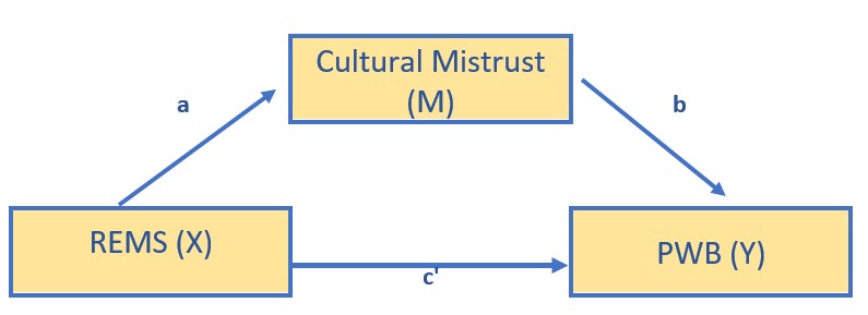
For the lessons on measurement and structural models, we will evaluate a simple mediation model, predicting psychological well-being from racial ethnic microaggressions through cultural mistrust.
9.5.1 Simulating the data from the journal article
We used the lavaan::simulateData function for the simulation. If you have taken psychometrics, you may recognize the code as one that creates latent variables form item-level data. In trying to be as authentic as possible, we retrieved factor loadings from psychometrically oriented articles that evaluated the measures (Nadal, 2011; Veit & Ware, 1983). For all others we specified a factor loading of 0.80. We then approximated the measurement model by specifying the correlations between all of the latent variable. We sourced these from the correlation matrix from the research vignette (Paul Youngbin Kim et al., 2017). The process created data with multiple decimals and values that exceeded the boundaries of the variables. For example, in all scales there were negative values. Therefore, the final element of the simulation was a linear transformation that rescaled the variables back to the range described in the journal article and rounding the values to integer (i.e., with no decimal places).
#Entering the intercorrelations, means, and standard deviations from the journal article
Kim_generating_model <- '
        #measurement model
         REMS =~ .82*Inf32 + .75*Inf38 + .74*Inf21 + .72*Inf17 + .69*Inf9 + .61*Inf36 + .51*Inf5 + .49*Inf22 + .81*SClass6 + .81*SClass31 + .74*SClass8 + .74*SClass40 + .72*SClass2 + .65*SClass34 + .55*SClass11 + .84*mInv27 + .84*mInv30 + .80*mInv39 + .72*mInv7 + .62*mInv26 + .61*mInv33 + .53*mInv4 + .47*mInv14 + .47*mInv10 + .74*Exot3 + .74*Exot29 + .71*Exot45 + .69*Exot35 + .60*Exot42 + .59*Exot23 + .51*Exot13 + .51*Exot20 + .49*Exot43 + .84*mEnv37 + .85*mEnv24 + .78*mEnv19 + .70*mEnv28 + .69*mEnv18 + .55*mEnv41 + .55*mEnv12 + .76*mWork25 + .67*mWork15 + .65*mWork1 + .64*mWork16 + .62*mWork44

         CMI =~ .8*cmi1 + .8*cmi2 + .8*cmi3 + .8*cmi4 + .8*cmi5 + .8*cmi6 + .8*cmi7 + .8*cmi8 + .8*cmi9 + .8*cmi10 + .8*cmi11 + .8*cmi12 + .8*cmi13 + .8*cmi14 + .8*cmi15 + .8*cmi16 + .8*cmi17 + .8*cmi18 + .8*cmi19 + .8*cmi20 + .8*cmi21 + .8*cmi22 + .8*cmi23 + .8*cmi24 + .8*cmi25 + .8*cmi26 + .8*cmi27 + .8*cmi28 + .8*cmi29 + .8*cmi30 + .8*cmi31 + .8*cmi32 + .8*cmi33 + .8*cmi34 + .8*cmi35 + .8*cmi36 + .8*cmi37 + .8*cmi38 + .8*cmi39 + .8*cmi40 + .8*cmi41 + .8*cmi42 + .8*cmi43 + .8*cmi44 + .8*cmi45 + .8*cmi46 + .8*cmi47

         ANX =~ .80*Anx1 + .80*Anx2 + .77*Anx3 + .74*Anx4 + .74*Anx5 + .69*Anx6 + .69*Anx7 + .68*Anx8 + .50*Anx9
         DEP =~ .74*Dep1 + .83*Dep2 + .82*Dep3 + .74*Dep4
         PWB =~ .83*pwb1 + .72*pwb2 + .67*pwb3 + .79*pwb4 + .77*pwb5 + .75*pwb6 + .74*pwb7 +.71*pwb8 +.67*pwb9 +.61*pwb10 +.58*pwb11

         HlpSkg =~ .8*hlpskg1 + .8*hlpskg2 + .8*hlpskg3 + .8*hlpskg4 + .8*hlpskg5 + .8*hlpskg6 + .8*hlpskg7 + .8*hlpskg8 + .8*hlpskg9 + .8*hlpskg10

        #Means
         REMS ~ 0.34*1
         CMI ~ 3*1
         ANX ~ 2.98*1
         DEP ~ 2.36*1
         PWB ~ 3.5*1
         HlpSkg ~ 1.64*1

        #Correlations
         REMS ~ 0.58*CMI
         REMS ~ 0.26*ANX
         REMS ~ 0.34*DEP
         REMS ~ -0.25*PWB
         REMS ~ -0.02*HlpSkg
         CMI ~ 0.12*ANX
         CMI ~ 0.19*DEP
         CMI ~ -0.28*PWB
         CMI ~ 0*HlpSkg
         ANX ~ 0.66*DEP
         ANX ~ -0.55*PWB
         ANX ~ 0.07*HlpSkg
         DEP ~ -0.66*PWB
         DEP ~ 0.05*HlpSkg
         PWB ~ 0.08*HlpSkg
        '

set.seed(230916)
dfKim <- lavaan::simulateData(model = Kim_generating_model,
                              model.type = "sem",
                              meanstructure = T,
                              sample.nobs=156,
                              standardized=FALSE)
library(tidyverse)

#used to retrieve column indices used in the rescaling script below
col_index <- as.data.frame(colnames(dfKim))

#for loop to go through each column of the dataframe
#1 thru 45 apply only to REMS variables
#46 thru 92 apply only to CMI variables
#93 thru 116 apply only to mental health variables
#117 thru 126 apply only to HlpSkng variables
for(i in 1:ncol(dfKim)){
  if(i >= 1 & i <= 45){
    dfKim[,i] <- scales::rescale(dfKim[,i], c(0, 1))
  }
  if(i >= 46 & i <= 92){
    dfKim[,i] <- scales::rescale(dfKim[,i], c(1, 7))
  }
  if(i >= 93 & i <= 116){
    dfKim[,i] <- scales::rescale(dfKim[,i], c(1, 5))
  }
  if(i >= 117 & i <= 126){
    dfKim[,i] <- scales::rescale(dfKim[,i], c(0, 3))
  }
}

#psych::describe(dfKim)+

library(tidyverse)
dfKim <- dfKim %>% round(0)

#I tested the rescaling the correlation between original and rescaled variables is 1.0
#Kim_df_latent$INF32 <- scales::rescale(Kim_df_latent$Inf32, c(0, 1))
#cor.test(Kim_df_latent$Inf32, Kim_df_latent$INF32, method="pearson")

#Checking our work against the original correlation matrix
#round(cor(Kim_df),3)
The script below allows you to store the simulated data as a file on your computer. This is optional – the entire lesson can be worked with the simulated data.
If you prefer the .rds format, use this script (remove the hashtags). The .rds format has the advantage of preserving any formatting of variables. A disadvantage is that you cannot open these files outside of the R environment.
Script to save the data to your computer as an .rds file.
Once saved, you could clean your environment and bring the data back in from its .csv format.
If you prefer the .csv format (think “Excel lite”) use this script (remove the hashtags). An advantage of the .csv format is that you can open the data outside of the R environment. A disadvantage is that it may not retain any formatting of variables
Script to save the data to your computer as a .csv file.
Once saved, you could clean your environment and bring the data back in from its .csv format.
9.6 Scrubbing, Scoring, and Data Diagnostics
Because the focus of this lesson is on the specific topic of establishing a measurement model for SEM and have used simulated data, we can skip many of the steps in scrubbing, scoring and data diagnostics. If this were real, raw, data, it would be important to scrub, if needed score, and conduct data diagnostics to evaluate the suitability of the data for the proposes anlayses.
9.7 Specifying the Measurement Model in lavaan
SEM in lavaan requires fluency with the R script:
- Latent variables (factors) must be defined by their manifest or latent indicators.
- the special operator (=~, is measured/defined by) is used for this
- Example: f1 =~ y1 + y2 + y3
- Regression equations use the single tilda (~, is regressed on)
- place DV (y) on left of operator
- place IVs, separate by + on the right
- Example: y ~ f1 + f2 + x1 + x2
- f is a latent variable in this example
- y, x1, and x2 are observed variables in this example
- An asterisk can affix a label in subsequent calculations and in interpreting output
- Variances and covariances are specified with a double tilde operator (~~, is correlated with)
- Example of variance: y1 ~~ y1 (the relationship with itself)
- Example of covariance: y1 ~~ y2 (relationship with another variable)
- Example of covariance of a factor: f1 ~~ f2 *Intercepts (~ 1) for observed and LVs are simple, intercept-only regression formulas
- Example of variable intercept: y1 ~ 1
- Example of factor intercept: f1 ~ 1
A complete lavaan model is a combination of these formula types, enclosed between single quotation models. Readibility of model syntax is improved by:
- splitting formulas over multiple lines
- using blank lines within single quote
- labeling with the hashtag
init_msmt_mod <- "
        ##measurement model
         REMS =~ Inf32 + Inf38 + Inf21 + Inf17 + Inf9 + Inf36 + Inf5 + Inf22 + SClass6 + SClass31 + SClass8 + SClass40 + SClass2 + SClass34 + SClass11 + mInv27 + mInv30 + mInv39 + mInv7 + mInv26 + mInv33 + mInv4 + mInv14 + mInv10 + Exot3 + Exot29 + Exot45 + Exot35 + Exot42 + Exot23 + Exot13 + Exot20 + Exot43 + mEnv37 + mEnv24 + mEnv19 + mEnv28 + mEnv18 + mEnv41 + mEnv12 + mWork25 + mWork15 + mWork1 + mWork16 + mWork44

         CMI =~ cmi1 + cmi2 + cmi3 + cmi4 + cmi5 + cmi6 + cmi7 + cmi8 + cmi9 + cmi10 + cmi11 + cmi12 + cmi13 + cmi14 + cmi15 + cmi16 + cmi17 + cmi18 + cmi19 + cmi20 + cmi21 + cmi22 + cmi23 + cmi24 + cmi25 + cmi26 + cmi27 + cmi28 + cmi29 + cmi30 + cmi31 + cmi32 + cmi33 + cmi34 + cmi35 + cmi36 + cmi37 + cmi38 + cmi39 + cmi40 + cmi41 + cmi42 + cmi43 + cmi44 + cmi45 + cmi46 + cmi47

         PWB =~ pwb1 + pwb2 + pwb3 + pwb4 + pwb5 + pwb6 + pwb7 + pwb8 + pwb9 + pwb10 + pwb11


        # Covariances
         REMS ~~ CMI
         REMS ~~ PWB
         CMI ~~ PWB
        "

set.seed(230916)
init_msmt_fit <- lavaan::cfa(init_msmt_mod, data = dfKim)
# you can add missing = 'fiml' to the code; I deleted it because it
# was really slowing down the run
init_msmt_fit_sum <- lavaan::summary(init_msmt_fit, fit.measures = TRUE,
    standardized = TRUE)
init_msmt_fit_sum
## lavaan 0.6.17 ended normally after 118 iterations
##
## Estimator ML
## Optimization method NLMINB
## Number of model parameters 209
##
## Number of observations 156
##
## Model Test User Model:
##
## Test statistic 7271.391
## Degrees of freedom 5147
## P-value (Chi-square) 0.000
##
## Model Test Baseline Model:
##
## Test statistic 13555.967
## Degrees of freedom 5253
## P-value 0.000
##
## User Model versus Baseline Model:
##
## Comparative Fit Index (CFI) 0.744
## Tucker-Lewis Index (TLI) 0.739
##
## Loglikelihood and Information Criteria:
##
## Loglikelihood user model (H0) -15294.957
## Loglikelihood unrestricted model (H1) -11659.262
##
## Akaike (AIC) 31007.915
## Bayesian (BIC) 31645.335
## Sample-size adjusted Bayesian (SABIC) 30983.784
##
## Root Mean Square Error of Approximation:
##
## RMSEA 0.051
## 90 Percent confidence interval - lower 0.049
## 90 Percent confidence interval - upper 0.054
## P-value H_0: RMSEA <= 0.050 0.193
## P-value H_0: RMSEA >= 0.080 0.000
##
## Standardized Root Mean Square Residual:
##
## SRMR 0.061
##
## Parameter Estimates:
##
## Standard errors Standard
## Information Expected
## Information saturated (h1) model Structured
##
## Latent Variables:
## Estimate Std.Err z-value P(>|z|) Std.lv Std.all
## REMS =~
## Inf32 1.000 0.282 0.572
## Inf38 1.063 0.169 6.289 0.000 0.300 0.606
## Inf21 0.894 0.151 5.935 0.000 0.252 0.560
## Inf17 0.970 0.165 5.871 0.000 0.273 0.552
## Inf9 1.010 0.163 6.213 0.000 0.285 0.596
## Inf36 1.026 0.169 6.079 0.000 0.289 0.579
## Inf5 0.907 0.156 5.811 0.000 0.256 0.545
## Inf22 0.945 0.165 5.711 0.000 0.266 0.533
## SClass6 1.146 0.173 6.631 0.000 0.323 0.654
## SClass31 1.039 0.169 6.133 0.000 0.293 0.586
## SClass8 0.893 0.150 5.959 0.000 0.252 0.563
## SClass40 1.036 0.168 6.184 0.000 0.292 0.592
## SClass2 0.963 0.164 5.855 0.000 0.271 0.550
## SClass34 0.949 0.161 5.882 0.000 0.268 0.554
## SClass11 0.867 0.162 5.345 0.000 0.244 0.489
## mInv27 1.045 0.168 6.232 0.000 0.294 0.599
## mInv30 0.970 0.158 6.133 0.000 0.273 0.586
## mInv39 1.143 0.174 6.573 0.000 0.322 0.645
## mInv7 0.946 0.161 5.868 0.000 0.267 0.552
## mInv26 1.122 0.173 6.483 0.000 0.316 0.633
## mInv33 1.080 0.166 6.516 0.000 0.305 0.637
## mInv4 0.744 0.147 5.060 0.000 0.210 0.457
## mInv14 0.910 0.150 6.075 0.000 0.256 0.578
## mInv10 0.817 0.159 5.130 0.000 0.230 0.465
## Exot3 1.164 0.174 6.673 0.000 0.328 0.660
## Exot29 1.092 0.169 6.455 0.000 0.308 0.629
## Exot45 1.099 0.172 6.389 0.000 0.310 0.620
## Exot35 1.103 0.168 6.559 0.000 0.311 0.643
## Exot42 1.000 0.167 5.998 0.000 0.282 0.568
## Exot23 0.862 0.154 5.589 0.000 0.243 0.518
## Exot13 0.761 0.150 5.079 0.000 0.214 0.459
## Exot20 0.805 0.158 5.087 0.000 0.227 0.460
## Exot43 0.671 0.139 4.840 0.000 0.189 0.433
## mEnv37 1.052 0.164 6.412 0.000 0.296 0.623
## mEnv24 1.248 0.178 7.002 0.000 0.352 0.709
## mEnv19 1.186 0.176 6.757 0.000 0.334 0.672
## mEnv28 0.931 0.164 5.671 0.000 0.262 0.528
## mEnv18 1.068 0.171 6.258 0.000 0.301 0.602
## mEnv41 0.972 0.166 5.861 0.000 0.274 0.551
## mEnv12 0.870 0.162 5.373 0.000 0.245 0.493
## mWork25 1.111 0.172 6.461 0.000 0.313 0.630
## mWork15 1.146 0.170 6.747 0.000 0.323 0.671
## mWork1 1.065 0.170 6.260 0.000 0.300 0.602
## mWork16 0.932 0.165 5.652 0.000 0.263 0.525
## mWork44 0.952 0.165 5.773 0.000 0.268 0.540
## CMI =~
## cmi1 1.000 0.767 0.654
## cmi2 0.945 0.128 7.373 0.000 0.725 0.639
## cmi3 1.006 0.126 7.995 0.000 0.772 0.702
## cmi4 0.979 0.129 7.618 0.000 0.751 0.664
## cmi5 0.958 0.131 7.339 0.000 0.735 0.636
## cmi6 0.914 0.123 7.459 0.000 0.701 0.648
## cmi7 1.003 0.136 7.380 0.000 0.769 0.640
## cmi8 1.083 0.140 7.739 0.000 0.831 0.676
## cmi9 0.953 0.133 7.191 0.000 0.731 0.621
## cmi10 0.993 0.129 7.711 0.000 0.762 0.673
## cmi11 0.990 0.122 8.083 0.000 0.759 0.711
## cmi12 1.089 0.142 7.646 0.000 0.836 0.666
## cmi13 1.066 0.144 7.403 0.000 0.818 0.642
## cmi14 1.018 0.137 7.418 0.000 0.781 0.644
## cmi15 0.865 0.121 7.154 0.000 0.663 0.618
## cmi16 0.971 0.138 7.032 0.000 0.745 0.606
## cmi17 1.102 0.146 7.522 0.000 0.846 0.654
## cmi18 1.042 0.138 7.557 0.000 0.800 0.658
## cmi19 0.940 0.130 7.240 0.000 0.722 0.626
## cmi20 0.835 0.118 7.085 0.000 0.641 0.611
## cmi21 0.813 0.111 7.330 0.000 0.623 0.635
## cmi22 0.991 0.128 7.723 0.000 0.760 0.674
## cmi23 0.970 0.143 6.782 0.000 0.745 0.582
## cmi24 0.952 0.129 7.376 0.000 0.730 0.640
## cmi25 1.053 0.142 7.433 0.000 0.808 0.645
## cmi26 0.811 0.126 6.455 0.000 0.622 0.551
## cmi27 1.029 0.130 7.939 0.000 0.790 0.696
## cmi28 0.995 0.127 7.810 0.000 0.764 0.683
## cmi29 0.784 0.123 6.378 0.000 0.602 0.543
## cmi30 0.993 0.131 7.608 0.000 0.762 0.663
## cmi31 1.010 0.133 7.601 0.000 0.775 0.662
## cmi32 1.051 0.131 8.036 0.000 0.806 0.706
## cmi33 1.094 0.137 7.971 0.000 0.840 0.699
## cmi34 1.035 0.138 7.492 0.000 0.794 0.651
## cmi35 0.938 0.134 7.024 0.000 0.720 0.605
## cmi36 0.842 0.125 6.730 0.000 0.646 0.577
## cmi37 0.990 0.147 6.754 0.000 0.760 0.579
## cmi38 1.129 0.147 7.663 0.000 0.866 0.668
## cmi39 0.985 0.128 7.692 0.000 0.756 0.671
## cmi40 1.181 0.145 8.124 0.000 0.906 0.715
## cmi41 1.007 0.131 7.697 0.000 0.773 0.672
## cmi42 1.082 0.139 7.775 0.000 0.830 0.679
## cmi43 1.205 0.144 8.397 0.000 0.925 0.744
## cmi44 0.880 0.118 7.435 0.000 0.675 0.645
## cmi45 0.922 0.120 7.672 0.000 0.708 0.669
## cmi46 0.926 0.137 6.778 0.000 0.711 0.581
## cmi47 1.139 0.164 6.942 0.000 0.874 0.597
## PWB =~
## pwb1 1.000 0.516 0.619
## pwb2 1.070 0.158 6.752 0.000 0.551 0.697
## pwb3 0.552 0.134 4.112 0.000 0.285 0.380
## pwb4 0.607 0.127 4.766 0.000 0.313 0.449
## pwb5 0.931 0.154 6.032 0.000 0.480 0.598
## pwb6 0.722 0.132 5.476 0.000 0.372 0.529
## pwb7 0.550 0.136 4.035 0.000 0.284 0.372
## pwb8 0.708 0.137 5.161 0.000 0.365 0.493
## pwb9 0.642 0.126 5.091 0.000 0.331 0.485
## pwb10 1.006 0.167 6.017 0.000 0.519 0.596
## pwb11 0.573 0.147 3.890 0.000 0.296 0.357
##
## Covariances:
## Estimate Std.Err z-value P(>|z|) Std.lv Std.all
## REMS ~~
## CMI 0.130 0.028 4.584 0.000 0.601 0.601
## PWB -0.081 0.019 -4.177 0.000 -0.559 -0.559
## CMI ~~
## PWB -0.225 0.051 -4.415 0.000 -0.568 -0.568
##
## Variances:
## Estimate Std.Err z-value P(>|z|) Std.lv Std.all
## .Inf32 0.164 0.019 8.653 0.000 0.164 0.673
## .Inf38 0.154 0.018 8.618 0.000 0.154 0.632
## .Inf21 0.139 0.016 8.663 0.000 0.139 0.686
## .Inf17 0.170 0.020 8.670 0.000 0.170 0.695
## .Inf9 0.147 0.017 8.629 0.000 0.147 0.645
## .Inf36 0.166 0.019 8.646 0.000 0.166 0.665
## .Inf5 0.155 0.018 8.676 0.000 0.155 0.703
## .Inf22 0.179 0.021 8.686 0.000 0.179 0.716
## .SClass6 0.140 0.016 8.557 0.000 0.140 0.573
## .SClass31 0.164 0.019 8.640 0.000 0.164 0.657
## .SClass8 0.136 0.016 8.661 0.000 0.136 0.683
## .SClass40 0.158 0.018 8.633 0.000 0.158 0.649
## .SClass2 0.169 0.020 8.672 0.000 0.169 0.697
## .SClass34 0.162 0.019 8.669 0.000 0.162 0.693
## .SClass11 0.190 0.022 8.716 0.000 0.190 0.761
## .mInv27 0.155 0.018 8.626 0.000 0.155 0.642
## .mInv30 0.143 0.017 8.640 0.000 0.143 0.657
## .mInv39 0.145 0.017 8.569 0.000 0.145 0.583
## .mInv7 0.162 0.019 8.671 0.000 0.162 0.695
## .mInv26 0.150 0.017 8.586 0.000 0.150 0.600
## .mInv33 0.136 0.016 8.580 0.000 0.136 0.594
## .mInv4 0.166 0.019 8.734 0.000 0.166 0.791
## .mInv14 0.131 0.015 8.647 0.000 0.131 0.666
## .mInv10 0.192 0.022 8.730 0.000 0.192 0.784
## .Exot3 0.140 0.016 8.548 0.000 0.140 0.565
## .Exot29 0.145 0.017 8.591 0.000 0.145 0.604
## .Exot45 0.154 0.018 8.602 0.000 0.154 0.616
## .Exot35 0.137 0.016 8.572 0.000 0.137 0.586
## .Exot42 0.166 0.019 8.656 0.000 0.166 0.677
## .Exot23 0.161 0.019 8.697 0.000 0.161 0.732
## .Exot13 0.172 0.020 8.733 0.000 0.172 0.789
## .Exot20 0.192 0.022 8.733 0.000 0.192 0.788
## .Exot43 0.155 0.018 8.747 0.000 0.155 0.812
## .mEnv37 0.138 0.016 8.598 0.000 0.138 0.612
## .mEnv24 0.122 0.014 8.459 0.000 0.122 0.497
## .mEnv19 0.136 0.016 8.529 0.000 0.136 0.548
## .mEnv28 0.178 0.021 8.690 0.000 0.178 0.721
## .mEnv18 0.159 0.018 8.622 0.000 0.159 0.637
## .mEnv41 0.172 0.020 8.671 0.000 0.172 0.696
## .mEnv12 0.188 0.022 8.714 0.000 0.188 0.757
## .mWork25 0.149 0.017 8.590 0.000 0.149 0.603
## .mWork15 0.128 0.015 8.531 0.000 0.128 0.550
## .mWork1 0.158 0.018 8.622 0.000 0.158 0.637
## .mWork16 0.181 0.021 8.691 0.000 0.181 0.724
## .mWork44 0.175 0.020 8.680 0.000 0.175 0.708
## .cmi1 0.789 0.091 8.647 0.000 0.789 0.573
## .cmi2 0.760 0.088 8.660 0.000 0.760 0.591
## .cmi3 0.614 0.071 8.591 0.000 0.614 0.507
## .cmi4 0.717 0.083 8.636 0.000 0.717 0.560
## .cmi5 0.797 0.092 8.663 0.000 0.797 0.596
## .cmi6 0.681 0.079 8.652 0.000 0.681 0.580
## .cmi7 0.853 0.099 8.660 0.000 0.853 0.591
## .cmi8 0.821 0.095 8.623 0.000 0.821 0.543
## .cmi9 0.851 0.098 8.676 0.000 0.851 0.614
## .cmi10 0.700 0.081 8.626 0.000 0.700 0.547
## .cmi11 0.564 0.066 8.578 0.000 0.564 0.495
## .cmi12 0.874 0.101 8.633 0.000 0.874 0.556
## .cmi13 0.953 0.110 8.657 0.000 0.953 0.588
## .cmi14 0.862 0.100 8.656 0.000 0.862 0.586
## .cmi15 0.713 0.082 8.679 0.000 0.713 0.618
## .cmi16 0.958 0.110 8.688 0.000 0.958 0.633
## .cmi17 0.956 0.111 8.646 0.000 0.956 0.572
## .cmi18 0.839 0.097 8.643 0.000 0.839 0.568
## .cmi19 0.807 0.093 8.672 0.000 0.807 0.608
## .cmi20 0.689 0.079 8.684 0.000 0.689 0.627
## .cmi21 0.575 0.066 8.664 0.000 0.575 0.597
## .cmi22 0.693 0.080 8.625 0.000 0.693 0.545
## .cmi23 1.084 0.125 8.705 0.000 1.084 0.662
## .cmi24 0.771 0.089 8.660 0.000 0.771 0.591
## .cmi25 0.915 0.106 8.655 0.000 0.915 0.584
## .cmi26 0.889 0.102 8.724 0.000 0.889 0.697
## .cmi27 0.663 0.077 8.598 0.000 0.663 0.515
## .cmi28 0.667 0.077 8.615 0.000 0.667 0.534
## .cmi29 0.864 0.099 8.728 0.000 0.864 0.705
## .cmi30 0.741 0.086 8.637 0.000 0.741 0.561
## .cmi31 0.770 0.089 8.638 0.000 0.770 0.562
## .cmi32 0.654 0.076 8.585 0.000 0.654 0.501
## .cmi33 0.736 0.086 8.594 0.000 0.736 0.511
## .cmi34 0.858 0.099 8.649 0.000 0.858 0.576
## .cmi35 0.897 0.103 8.688 0.000 0.897 0.634
## .cmi36 0.838 0.096 8.708 0.000 0.838 0.667
## .cmi37 1.144 0.131 8.706 0.000 1.144 0.665
## .cmi38 0.931 0.108 8.631 0.000 0.931 0.554
## .cmi39 0.697 0.081 8.628 0.000 0.697 0.550
## .cmi40 0.783 0.091 8.572 0.000 0.783 0.488
## .cmi41 0.727 0.084 8.628 0.000 0.727 0.549
## .cmi42 0.803 0.093 8.619 0.000 0.803 0.538
## .cmi43 0.690 0.081 8.524 0.000 0.690 0.447
## .cmi44 0.638 0.074 8.654 0.000 0.638 0.583
## .cmi45 0.618 0.072 8.630 0.000 0.618 0.552
## .cmi46 0.989 0.114 8.705 0.000 0.989 0.662
## .cmi47 1.378 0.159 8.694 0.000 1.378 0.643
## .pwb1 0.428 0.055 7.736 0.000 0.428 0.617
## .pwb2 0.322 0.045 7.163 0.000 0.322 0.514
## .pwb3 0.481 0.056 8.537 0.000 0.481 0.856
## .pwb4 0.389 0.046 8.389 0.000 0.389 0.799
## .pwb5 0.415 0.053 7.853 0.000 0.415 0.643
## .pwb6 0.356 0.044 8.148 0.000 0.356 0.720
## .pwb7 0.502 0.059 8.551 0.000 0.502 0.862
## .pwb8 0.415 0.050 8.269 0.000 0.415 0.757
## .pwb9 0.356 0.043 8.292 0.000 0.356 0.765
## .pwb10 0.489 0.062 7.863 0.000 0.489 0.645
## .pwb11 0.598 0.070 8.576 0.000 0.598 0.873
## REMS 0.079 0.021 3.838 0.000 1.000 1.000
## CMI 0.589 0.129 4.555 0.000 1.000 1.000
## PWB 0.266 0.067 3.949 0.000 1.000 1.000Evaluating our measurement model involves inspection of (a) the strength, significance, and direction of each of the indicators on their respective factors, (b) the global fit indices, and (c) the direction and degree to which the factors are correlated. While these three are the big buckets of evaluation, the lavaan::cfa output is rich with information.
If you wish to export the results for creation of tables, tidySEM has a number of functions that make this helpful. When you feed them to an object, the object can be downloaded as a .csv file
The tidySEM::table_fit function will display all of the global fit indices.
## Registered S3 method overwritten by 'tidySEM':
##   method          from
## predict.MxModel OpenMx## Name Parameters fmin chisq df pvalue baseline.chisq
## 1 init_msmt_fit 209 23.30574 7271.391 5147 0 13555.97
## baseline.df baseline.pvalue cfi tli nnfi rfi nfi
## 1 5253 0 0.7441408 0.7388715 0.7388715 0.4525554 0.4636022
## pnfi ifi rni LL unrestricted.logl aic bic
## 1 0.4542472 0.7473661 0.7441408 -15294.96 -11659.26 31007.91 31645.33
## n bic2 rmsea rmsea.ci.lower rmsea.ci.upper rmsea.ci.level
## 1 156 30983.78 0.05143726 0.04868226 0.05414449 0.9
## rmsea.pvalue rmsea.close.h0
## 1 0.1931555 0.05
## rmsea.notclose.pvalue
## 1 0.00000000000000000000000000000000000000000000000000000000000000000000000000000002002323
## rmsea.notclose.h0 rmr rmr_nomean srmr srmr_bentler
## 1 0.08 0.04292907 0.04292907 0.06061422 0.06061422
## srmr_bentler_nomean crmr crmr_nomean srmr_mplus srmr_mplus_nomean
## 1 0.06061422 0.0612056 0.0612056 0.06061422 0.06061422
## cn_05 cn_01 gfi agfi pgfi mfi ecvi
## 1 115.028 116.5502 0.598818 0.5825275 0.5754511 0.001103858 49.29096The tidySEM::table_results function produces all of the factor loadings, covariances, and variances,
init_msmt_pEsts <- tidySEM::table_results(init_msmt_fit, digits = 3, columns = NULL)
init_msmt_pEsts
## lhs op rhs est se pval confint est_sig est_std
## 1 REMS =~ Inf32 1.000 0.000 <NA> [1.000, 1.000] 1.000 0.572
## 2 REMS =~ Inf38 1.063 0.169 0.000 [0.731, 1.394] 1.063*** 0.606
## 3 REMS =~ Inf21 0.894 0.151 0.000 [0.599, 1.190] 0.894*** 0.560
## 4 REMS =~ Inf17 0.970 0.165 0.000 [0.646, 1.294] 0.970*** 0.552
## 5 REMS =~ Inf9 1.010 0.163 0.000 [0.692, 1.329] 1.010*** 0.596
## 6 REMS =~ Inf36 1.026 0.169 0.000 [0.695, 1.357] 1.026*** 0.579
## 7 REMS =~ Inf5 0.907 0.156 0.000 [0.601, 1.213] 0.907*** 0.545
## 8 REMS =~ Inf22 0.945 0.165 0.000 [0.620, 1.269] 0.945*** 0.533
## 9 REMS =~ SClass6 1.146 0.173 0.000 [0.807, 1.485] 1.146*** 0.654
## 10 REMS =~ SClass31 1.039 0.169 0.000 [0.707, 1.371] 1.039*** 0.586
## 11 REMS =~ SClass8 0.893 0.150 0.000 [0.599, 1.187] 0.893*** 0.563
## 12 REMS =~ SClass40 1.036 0.168 0.000 [0.708, 1.364] 1.036*** 0.592
## 13 REMS =~ SClass2 0.963 0.164 0.000 [0.640, 1.285] 0.963*** 0.550
## 14 REMS =~ SClass34 0.949 0.161 0.000 [0.633, 1.266] 0.949*** 0.554
## 15 REMS =~ SClass11 0.867 0.162 0.000 [0.549, 1.185] 0.867*** 0.489
## 16 REMS =~ mInv27 1.045 0.168 0.000 [0.716, 1.373] 1.045*** 0.599
## 17 REMS =~ mInv30 0.970 0.158 0.000 [0.660, 1.280] 0.970*** 0.586
## 18 REMS =~ mInv39 1.143 0.174 0.000 [0.802, 1.483] 1.143*** 0.645
## 19 REMS =~ mInv7 0.946 0.161 0.000 [0.630, 1.262] 0.946*** 0.552
## 20 REMS =~ mInv26 1.122 0.173 0.000 [0.782, 1.461] 1.122*** 0.633
## 21 REMS =~ mInv33 1.080 0.166 0.000 [0.755, 1.405] 1.080*** 0.637
## 22 REMS =~ mInv4 0.744 0.147 0.000 [0.456, 1.033] 0.744*** 0.457
## 23 REMS =~ mInv14 0.910 0.150 0.000 [0.616, 1.203] 0.910*** 0.578
## 24 REMS =~ mInv10 0.817 0.159 0.000 [0.505, 1.129] 0.817*** 0.465
## 25 REMS =~ Exot3 1.164 0.174 0.000 [0.822, 1.506] 1.164*** 0.660
## 26 REMS =~ Exot29 1.092 0.169 0.000 [0.760, 1.423] 1.092*** 0.629
## 27 REMS =~ Exot45 1.099 0.172 0.000 [0.762, 1.437] 1.099*** 0.620
## 28 REMS =~ Exot35 1.103 0.168 0.000 [0.774, 1.433] 1.103*** 0.643
## 29 REMS =~ Exot42 1.000 0.167 0.000 [0.673, 1.326] 1.000*** 0.568
## 30 REMS =~ Exot23 0.862 0.154 0.000 [0.560, 1.164] 0.862*** 0.518
## 31 REMS =~ Exot13 0.761 0.150 0.000 [0.467, 1.054] 0.761*** 0.459
## 32 REMS =~ Exot20 0.805 0.158 0.000 [0.495, 1.115] 0.805*** 0.460
## 33 REMS =~ Exot43 0.671 0.139 0.000 [0.399, 0.943] 0.671*** 0.433
## 34 REMS =~ mEnv37 1.052 0.164 0.000 [0.730, 1.373] 1.052*** 0.623
## 35 REMS =~ mEnv24 1.248 0.178 0.000 [0.898, 1.597] 1.248*** 0.709
## 36 REMS =~ mEnv19 1.186 0.176 0.000 [0.842, 1.530] 1.186*** 0.672
## 37 REMS =~ mEnv28 0.931 0.164 0.000 [0.609, 1.253] 0.931*** 0.528
## 38 REMS =~ mEnv18 1.068 0.171 0.000 [0.734, 1.403] 1.068*** 0.602
## 39 REMS =~ mEnv41 0.972 0.166 0.000 [0.647, 1.297] 0.972*** 0.551
## 40 REMS =~ mEnv12 0.870 0.162 0.000 [0.553, 1.188] 0.870*** 0.493
## 41 REMS =~ mWork25 1.111 0.172 0.000 [0.774, 1.448] 1.111*** 0.630
## 42 REMS =~ mWork15 1.146 0.170 0.000 [0.813, 1.478] 1.146*** 0.671
## 43 REMS =~ mWork1 1.065 0.170 0.000 [0.732, 1.399] 1.065*** 0.602
## 44 REMS =~ mWork16 0.932 0.165 0.000 [0.609, 1.255] 0.932*** 0.525
## 45 REMS =~ mWork44 0.952 0.165 0.000 [0.629, 1.275] 0.952*** 0.540
## 46 CMI =~ cmi1 1.000 0.000 <NA> [1.000, 1.000] 1.000 0.654
## 47 CMI =~ cmi2 0.945 0.128 0.000 [0.694, 1.196] 0.945*** 0.639
## 48 CMI =~ cmi3 1.006 0.126 0.000 [0.760, 1.253] 1.006*** 0.702
## 49 CMI =~ cmi4 0.979 0.129 0.000 [0.727, 1.231] 0.979*** 0.664
## 50 CMI =~ cmi5 0.958 0.131 0.000 [0.703, 1.214] 0.958*** 0.636
## 51 CMI =~ cmi6 0.914 0.123 0.000 [0.674, 1.154] 0.914*** 0.648
## 52 CMI =~ cmi7 1.003 0.136 0.000 [0.736, 1.269] 1.003*** 0.640
## 53 CMI =~ cmi8 1.083 0.140 0.000 [0.809, 1.358] 1.083*** 0.676
## 54 CMI =~ cmi9 0.953 0.133 0.000 [0.693, 1.213] 0.953*** 0.621
## 55 CMI =~ cmi10 0.993 0.129 0.000 [0.740, 1.245] 0.993*** 0.673
## 56 CMI =~ cmi11 0.990 0.122 0.000 [0.750, 1.230] 0.990*** 0.711
## 57 CMI =~ cmi12 1.089 0.142 0.000 [0.810, 1.369] 1.089*** 0.666
## 58 CMI =~ cmi13 1.066 0.144 0.000 [0.784, 1.348] 1.066*** 0.642
## 59 CMI =~ cmi14 1.018 0.137 0.000 [0.749, 1.287] 1.018*** 0.644
## 60 CMI =~ cmi15 0.865 0.121 0.000 [0.628, 1.101] 0.865*** 0.618
## 61 CMI =~ cmi16 0.971 0.138 0.000 [0.700, 1.242] 0.971*** 0.606
## 62 CMI =~ cmi17 1.102 0.146 0.000 [0.815, 1.389] 1.102*** 0.654
## 63 CMI =~ cmi18 1.042 0.138 0.000 [0.772, 1.312] 1.042*** 0.658
## 64 CMI =~ cmi19 0.940 0.130 0.000 [0.686, 1.195] 0.940*** 0.626
## 65 CMI =~ cmi20 0.835 0.118 0.000 [0.604, 1.066] 0.835*** 0.611
## 66 CMI =~ cmi21 0.813 0.111 0.000 [0.595, 1.030] 0.813*** 0.635
## 67 CMI =~ cmi22 0.991 0.128 0.000 [0.739, 1.242] 0.991*** 0.674
## 68 CMI =~ cmi23 0.970 0.143 0.000 [0.690, 1.251] 0.970*** 0.582
## 69 CMI =~ cmi24 0.952 0.129 0.000 [0.699, 1.205] 0.952*** 0.640
## 70 CMI =~ cmi25 1.053 0.142 0.000 [0.775, 1.330] 1.053*** 0.645
## 71 CMI =~ cmi26 0.811 0.126 0.000 [0.565, 1.057] 0.811*** 0.551
## 72 CMI =~ cmi27 1.029 0.130 0.000 [0.775, 1.283] 1.029*** 0.696
## 73 CMI =~ cmi28 0.995 0.127 0.000 [0.746, 1.245] 0.995*** 0.683
## 74 CMI =~ cmi29 0.784 0.123 0.000 [0.543, 1.026] 0.784*** 0.543
## 75 CMI =~ cmi30 0.993 0.131 0.000 [0.737, 1.249] 0.993*** 0.663
## 76 CMI =~ cmi31 1.010 0.133 0.000 [0.749, 1.270] 1.010*** 0.662
## 77 CMI =~ cmi32 1.051 0.131 0.000 [0.794, 1.307] 1.051*** 0.706
## 78 CMI =~ cmi33 1.094 0.137 0.000 [0.825, 1.363] 1.094*** 0.699
## 79 CMI =~ cmi34 1.035 0.138 0.000 [0.764, 1.306] 1.035*** 0.651
## 80 CMI =~ cmi35 0.938 0.134 0.000 [0.676, 1.200] 0.938*** 0.605
## 81 CMI =~ cmi36 0.842 0.125 0.000 [0.597, 1.088] 0.842*** 0.577
## 82 CMI =~ cmi37 0.990 0.147 0.000 [0.703, 1.277] 0.990*** 0.579
## 83 CMI =~ cmi38 1.129 0.147 0.000 [0.840, 1.418] 1.129*** 0.668
## 84 CMI =~ cmi39 0.985 0.128 0.000 [0.734, 1.236] 0.985*** 0.671
## 85 CMI =~ cmi40 1.181 0.145 0.000 [0.896, 1.465] 1.181*** 0.715
## 86 CMI =~ cmi41 1.007 0.131 0.000 [0.751, 1.264] 1.007*** 0.672
## 87 CMI =~ cmi42 1.082 0.139 0.000 [0.809, 1.354] 1.082*** 0.679
## 88 CMI =~ cmi43 1.205 0.144 0.000 [0.924, 1.486] 1.205*** 0.744
## 89 CMI =~ cmi44 0.880 0.118 0.000 [0.648, 1.111] 0.880*** 0.645
## 90 CMI =~ cmi45 0.922 0.120 0.000 [0.687, 1.158] 0.922*** 0.669
## 91 CMI =~ cmi46 0.926 0.137 0.000 [0.658, 1.194] 0.926*** 0.581
## 92 CMI =~ cmi47 1.139 0.164 0.000 [0.817, 1.461] 1.139*** 0.597
## 93 PWB =~ pwb1 1.000 0.000 <NA> [1.000, 1.000] 1.000 0.619
## 94 PWB =~ pwb2 1.070 0.158 0.000 [0.759, 1.380] 1.070*** 0.697
## 95 PWB =~ pwb3 0.552 0.134 0.000 [0.289, 0.815] 0.552*** 0.380
## 96 PWB =~ pwb4 0.607 0.127 0.000 [0.358, 0.857] 0.607*** 0.449
## 97 PWB =~ pwb5 0.931 0.154 0.000 [0.629, 1.234] 0.931*** 0.598
## 98 PWB =~ pwb6 0.722 0.132 0.000 [0.464, 0.980] 0.722*** 0.529
## 99 PWB =~ pwb7 0.550 0.136 0.000 [0.283, 0.818] 0.550*** 0.372
## 100 PWB =~ pwb8 0.708 0.137 0.000 [0.439, 0.977] 0.708*** 0.493
## 101 PWB =~ pwb9 0.642 0.126 0.000 [0.395, 0.889] 0.642*** 0.485
## 102 PWB =~ pwb10 1.006 0.167 0.000 [0.678, 1.334] 1.006*** 0.596
## 103 PWB =~ pwb11 0.573 0.147 0.000 [0.285, 0.862] 0.573*** 0.357
## 104 REMS ~~ CMI 0.130 0.028 0.000 [0.074, 0.186] 0.130*** 0.601
## 105 REMS ~~ PWB -0.081 0.019 0.000 [-0.119, -0.043] -0.081*** -0.559
## 106 CMI ~~ PWB -0.225 0.051 0.000 [-0.324, -0.125] -0.225*** -0.568
## 107 Inf32 ~~ Inf32 0.164 0.019 0.000 [0.127, 0.201] 0.164*** 0.673
## 108 Inf38 ~~ Inf38 0.154 0.018 0.000 [0.119, 0.189] 0.154*** 0.632
## 109 Inf21 ~~ Inf21 0.139 0.016 0.000 [0.107, 0.170] 0.139*** 0.686
## 110 Inf17 ~~ Inf17 0.170 0.020 0.000 [0.132, 0.209] 0.170*** 0.695
## 111 Inf9 ~~ Inf9 0.147 0.017 0.000 [0.114, 0.181] 0.147*** 0.645
## 112 Inf36 ~~ Inf36 0.166 0.019 0.000 [0.129, 0.204] 0.166*** 0.665
## 113 Inf5 ~~ Inf5 0.155 0.018 0.000 [0.120, 0.190] 0.155*** 0.703
## 114 Inf22 ~~ Inf22 0.179 0.021 0.000 [0.139, 0.219] 0.179*** 0.716
## 115 SClass6 ~~ SClass6 0.140 0.016 0.000 [0.108, 0.172] 0.140*** 0.573
## 116 SClass31 ~~ SClass31 0.164 0.019 0.000 [0.127, 0.202] 0.164*** 0.657
## 117 SClass8 ~~ SClass8 0.136 0.016 0.000 [0.105, 0.167] 0.136*** 0.683
## 118 SClass40 ~~ SClass40 0.158 0.018 0.000 [0.122, 0.194] 0.158*** 0.649
## 119 SClass2 ~~ SClass2 0.169 0.020 0.000 [0.131, 0.208] 0.169*** 0.697
## 120 SClass34 ~~ SClass34 0.162 0.019 0.000 [0.125, 0.199] 0.162*** 0.693
## 121 SClass11 ~~ SClass11 0.190 0.022 0.000 [0.147, 0.233] 0.190*** 0.761
## 122 mInv27 ~~ mInv27 0.155 0.018 0.000 [0.120, 0.191] 0.155*** 0.642
## 123 mInv30 ~~ mInv30 0.143 0.017 0.000 [0.111, 0.176] 0.143*** 0.657
## 124 mInv39 ~~ mInv39 0.145 0.017 0.000 [0.112, 0.178] 0.145*** 0.583
## 125 mInv7 ~~ mInv7 0.162 0.019 0.000 [0.126, 0.199] 0.162*** 0.695
## 126 mInv26 ~~ mInv26 0.150 0.017 0.000 [0.116, 0.184] 0.150*** 0.600
## 127 mInv33 ~~ mInv33 0.136 0.016 0.000 [0.105, 0.166] 0.136*** 0.594
## 128 mInv4 ~~ mInv4 0.166 0.019 0.000 [0.129, 0.204] 0.166*** 0.791
## 129 mInv14 ~~ mInv14 0.131 0.015 0.000 [0.101, 0.161] 0.131*** 0.666
## 130 mInv10 ~~ mInv10 0.192 0.022 0.000 [0.149, 0.235] 0.192*** 0.784
## 131 Exot3 ~~ Exot3 0.140 0.016 0.000 [0.108, 0.172] 0.140*** 0.565
## 132 Exot29 ~~ Exot29 0.145 0.017 0.000 [0.112, 0.178] 0.145*** 0.604
## 133 Exot45 ~~ Exot45 0.154 0.018 0.000 [0.119, 0.189] 0.154*** 0.616
## 134 Exot35 ~~ Exot35 0.137 0.016 0.000 [0.106, 0.168] 0.137*** 0.586
## 135 Exot42 ~~ Exot42 0.166 0.019 0.000 [0.129, 0.204] 0.166*** 0.677
## 136 Exot23 ~~ Exot23 0.161 0.019 0.000 [0.125, 0.197] 0.161*** 0.732
## 137 Exot13 ~~ Exot13 0.172 0.020 0.000 [0.133, 0.210] 0.172*** 0.789
## 138 Exot20 ~~ Exot20 0.192 0.022 0.000 [0.149, 0.235] 0.192*** 0.788
## 139 Exot43 ~~ Exot43 0.155 0.018 0.000 [0.120, 0.190] 0.155*** 0.812
## 140 mEnv37 ~~ mEnv37 0.138 0.016 0.000 [0.107, 0.170] 0.138*** 0.612
## 141 mEnv24 ~~ mEnv24 0.122 0.014 0.000 [0.094, 0.151] 0.122*** 0.497
## 142 mEnv19 ~~ mEnv19 0.136 0.016 0.000 [0.104, 0.167] 0.136*** 0.548
## 143 mEnv28 ~~ mEnv28 0.178 0.021 0.000 [0.138, 0.219] 0.178*** 0.721
## 144 mEnv18 ~~ mEnv18 0.159 0.018 0.000 [0.123, 0.196] 0.159*** 0.637
## 145 mEnv41 ~~ mEnv41 0.172 0.020 0.000 [0.133, 0.211] 0.172*** 0.696
## 146 mEnv12 ~~ mEnv12 0.188 0.022 0.000 [0.146, 0.230] 0.188*** 0.757
## 147 mWork25 ~~ mWork25 0.149 0.017 0.000 [0.115, 0.183] 0.149*** 0.603
## 148 mWork15 ~~ mWork15 0.128 0.015 0.000 [0.098, 0.157] 0.128*** 0.550
## 149 mWork1 ~~ mWork1 0.158 0.018 0.000 [0.122, 0.194] 0.158*** 0.637
## 150 mWork16 ~~ mWork16 0.181 0.021 0.000 [0.140, 0.222] 0.181*** 0.724
## 151 mWork44 ~~ mWork44 0.175 0.020 0.000 [0.135, 0.214] 0.175*** 0.708
## 152 cmi1 ~~ cmi1 0.789 0.091 0.000 [0.610, 0.968] 0.789*** 0.573
## 153 cmi2 ~~ cmi2 0.760 0.088 0.000 [0.588, 0.932] 0.760*** 0.591
## 154 cmi3 ~~ cmi3 0.614 0.071 0.000 [0.474, 0.754] 0.614*** 0.507
## 155 cmi4 ~~ cmi4 0.717 0.083 0.000 [0.555, 0.880] 0.717*** 0.560
## 156 cmi5 ~~ cmi5 0.797 0.092 0.000 [0.617, 0.977] 0.797*** 0.596
## 157 cmi6 ~~ cmi6 0.681 0.079 0.000 [0.526, 0.835] 0.681*** 0.580
## 158 cmi7 ~~ cmi7 0.853 0.099 0.000 [0.660, 1.047] 0.853*** 0.591
## 159 cmi8 ~~ cmi8 0.821 0.095 0.000 [0.635, 1.008] 0.821*** 0.543
## 160 cmi9 ~~ cmi9 0.851 0.098 0.000 [0.659, 1.043] 0.851*** 0.614
## 161 cmi10 ~~ cmi10 0.700 0.081 0.000 [0.541, 0.860] 0.700*** 0.547
## 162 cmi11 ~~ cmi11 0.564 0.066 0.000 [0.435, 0.693] 0.564*** 0.495
## 163 cmi12 ~~ cmi12 0.874 0.101 0.000 [0.676, 1.073] 0.874*** 0.556
## 164 cmi13 ~~ cmi13 0.953 0.110 0.000 [0.737, 1.169] 0.953*** 0.588
## 165 cmi14 ~~ cmi14 0.862 0.100 0.000 [0.667, 1.057] 0.862*** 0.586
## 166 cmi15 ~~ cmi15 0.713 0.082 0.000 [0.552, 0.874] 0.713*** 0.618
## 167 cmi16 ~~ cmi16 0.958 0.110 0.000 [0.742, 1.174] 0.958*** 0.633
## 168 cmi17 ~~ cmi17 0.956 0.111 0.000 [0.739, 1.173] 0.956*** 0.572
## 169 cmi18 ~~ cmi18 0.839 0.097 0.000 [0.649, 1.030] 0.839*** 0.568
## 170 cmi19 ~~ cmi19 0.807 0.093 0.000 [0.625, 0.990] 0.807*** 0.608
## 171 cmi20 ~~ cmi20 0.689 0.079 0.000 [0.534, 0.845] 0.689*** 0.627
## 172 cmi21 ~~ cmi21 0.575 0.066 0.000 [0.445, 0.705] 0.575*** 0.597
## 173 cmi22 ~~ cmi22 0.693 0.080 0.000 [0.536, 0.851] 0.693*** 0.545
## 174 cmi23 ~~ cmi23 1.084 0.125 0.000 [0.840, 1.328] 1.084*** 0.662
## 175 cmi24 ~~ cmi24 0.771 0.089 0.000 [0.596, 0.945] 0.771*** 0.591
## 176 cmi25 ~~ cmi25 0.915 0.106 0.000 [0.708, 1.122] 0.915*** 0.584
## 177 cmi26 ~~ cmi26 0.889 0.102 0.000 [0.690, 1.089] 0.889*** 0.697
## 178 cmi27 ~~ cmi27 0.663 0.077 0.000 [0.512, 0.814] 0.663*** 0.515
## 179 cmi28 ~~ cmi28 0.667 0.077 0.000 [0.515, 0.819] 0.667*** 0.534
## 180 cmi29 ~~ cmi29 0.864 0.099 0.000 [0.670, 1.058] 0.864*** 0.705
## 181 cmi30 ~~ cmi30 0.741 0.086 0.000 [0.573, 0.910] 0.741*** 0.561
## 182 cmi31 ~~ cmi31 0.770 0.089 0.000 [0.595, 0.945] 0.770*** 0.562
## 183 cmi32 ~~ cmi32 0.654 0.076 0.000 [0.504, 0.803] 0.654*** 0.501
## 184 cmi33 ~~ cmi33 0.736 0.086 0.000 [0.568, 0.904] 0.736*** 0.511
## 185 cmi34 ~~ cmi34 0.858 0.099 0.000 [0.663, 1.052] 0.858*** 0.576
## 186 cmi35 ~~ cmi35 0.897 0.103 0.000 [0.695, 1.100] 0.897*** 0.634
## 187 cmi36 ~~ cmi36 0.838 0.096 0.000 [0.649, 1.027] 0.838*** 0.667
## 188 cmi37 ~~ cmi37 1.144 0.131 0.000 [0.886, 1.401] 1.144*** 0.665
## 189 cmi38 ~~ cmi38 0.931 0.108 0.000 [0.719, 1.142] 0.931*** 0.554
## 190 cmi39 ~~ cmi39 0.697 0.081 0.000 [0.539, 0.856] 0.697*** 0.550
## 191 cmi40 ~~ cmi40 0.783 0.091 0.000 [0.604, 0.963] 0.783*** 0.488
## 192 cmi41 ~~ cmi41 0.727 0.084 0.000 [0.562, 0.893] 0.727*** 0.549
## 193 cmi42 ~~ cmi42 0.803 0.093 0.000 [0.621, 0.986] 0.803*** 0.538
## 194 cmi43 ~~ cmi43 0.690 0.081 0.000 [0.532, 0.849] 0.690*** 0.447
## 195 cmi44 ~~ cmi44 0.638 0.074 0.000 [0.494, 0.783] 0.638*** 0.583
## 196 cmi45 ~~ cmi45 0.618 0.072 0.000 [0.478, 0.758] 0.618*** 0.552
## 197 cmi46 ~~ cmi46 0.989 0.114 0.000 [0.766, 1.211] 0.989*** 0.662
## 198 cmi47 ~~ cmi47 1.378 0.159 0.000 [1.068, 1.689] 1.378*** 0.643
## 199 pwb1 ~~ pwb1 0.428 0.055 0.000 [0.319, 0.536] 0.428*** 0.617
## 200 pwb2 ~~ pwb2 0.322 0.045 0.000 [0.234, 0.410] 0.322*** 0.514
## 201 pwb3 ~~ pwb3 0.481 0.056 0.000 [0.371, 0.591] 0.481*** 0.856
## 202 pwb4 ~~ pwb4 0.389 0.046 0.000 [0.298, 0.479] 0.389*** 0.799
## 203 pwb5 ~~ pwb5 0.415 0.053 0.000 [0.311, 0.518] 0.415*** 0.643
## 204 pwb6 ~~ pwb6 0.356 0.044 0.000 [0.270, 0.442] 0.356*** 0.720
## 205 pwb7 ~~ pwb7 0.502 0.059 0.000 [0.387, 0.617] 0.502*** 0.862
## 206 pwb8 ~~ pwb8 0.415 0.050 0.000 [0.317, 0.514] 0.415*** 0.757
## 207 pwb9 ~~ pwb9 0.356 0.043 0.000 [0.272, 0.441] 0.356*** 0.765
## 208 pwb10 ~~ pwb10 0.489 0.062 0.000 [0.367, 0.611] 0.489*** 0.645
## 209 pwb11 ~~ pwb11 0.598 0.070 0.000 [0.462, 0.735] 0.598*** 0.873
## 210 REMS ~~ REMS 0.079 0.021 0.000 [0.039, 0.120] 0.079*** 1.000
## 211 CMI ~~ CMI 0.589 0.129 0.000 [0.335, 0.842] 0.589*** 1.000
## 212 PWB ~~ PWB 0.266 0.067 0.000 [0.134, 0.398] 0.266*** 1.000
## se_std pval_std confint_std est_sig_std label
## 1 0.056 0.000 [0.463, 0.681] 0.572*** REMS.BY.Inf32
## 2 0.052 0.000 [0.504, 0.709] 0.606*** REMS.BY.Inf38
## 3 0.057 0.000 [0.449, 0.671] 0.560*** REMS.BY.Inf21
## 4 0.057 0.000 [0.440, 0.665] 0.552*** REMS.BY.Inf17
## 5 0.053 0.000 [0.492, 0.701] 0.596*** REMS.BY.Inf9
## 6 0.055 0.000 [0.471, 0.686] 0.579*** REMS.BY.Inf36
## 7 0.058 0.000 [0.431, 0.659] 0.545*** REMS.BY.Inf5
## 8 0.059 0.000 [0.417, 0.648] 0.533*** REMS.BY.Inf22
## 9 0.048 0.000 [0.561, 0.747] 0.654*** REMS.BY.SClass6
## 10 0.054 0.000 [0.479, 0.692] 0.586*** REMS.BY.SClass31
## 11 0.056 0.000 [0.453, 0.674] 0.563*** REMS.BY.SClass8
## 12 0.054 0.000 [0.487, 0.698] 0.592*** REMS.BY.SClass40
## 13 0.058 0.000 [0.438, 0.663] 0.550*** REMS.BY.SClass2
## 14 0.057 0.000 [0.442, 0.666] 0.554*** REMS.BY.SClass34
## 15 0.063 0.000 [0.367, 0.612] 0.489*** REMS.BY.SClass11
## 16 0.053 0.000 [0.495, 0.703] 0.599*** REMS.BY.mInv27
## 17 0.054 0.000 [0.479, 0.692] 0.586*** REMS.BY.mInv30
## 18 0.048 0.000 [0.551, 0.740] 0.645*** REMS.BY.mInv39
## 19 0.057 0.000 [0.440, 0.664] 0.552*** REMS.BY.mInv7
## 20 0.050 0.000 [0.535, 0.730] 0.633*** REMS.BY.mInv26
## 21 0.049 0.000 [0.541, 0.734] 0.637*** REMS.BY.mInv33
## 22 0.065 0.000 [0.330, 0.585] 0.457*** REMS.BY.mInv4
## 23 0.055 0.000 [0.470, 0.686] 0.578*** REMS.BY.mInv14
## 24 0.064 0.000 [0.339, 0.591] 0.465*** REMS.BY.mInv10
## 25 0.047 0.000 [0.568, 0.752] 0.660*** REMS.BY.Exot3
## 26 0.050 0.000 [0.531, 0.727] 0.629*** REMS.BY.Exot29
## 27 0.051 0.000 [0.520, 0.720] 0.620*** REMS.BY.Exot45
## 28 0.049 0.000 [0.548, 0.739] 0.643*** REMS.BY.Exot35
## 29 0.056 0.000 [0.459, 0.678] 0.568*** REMS.BY.Exot42
## 30 0.060 0.000 [0.400, 0.636] 0.518*** REMS.BY.Exot23
## 31 0.065 0.000 [0.332, 0.586] 0.459*** REMS.BY.Exot13
## 32 0.065 0.000 [0.333, 0.587] 0.460*** REMS.BY.Exot20
## 33 0.067 0.000 [0.303, 0.564] 0.433*** REMS.BY.Exot43
## 34 0.051 0.000 [0.524, 0.722] 0.623*** REMS.BY.mEnv37
## 35 0.042 0.000 [0.628, 0.791] 0.709*** REMS.BY.mEnv24
## 36 0.046 0.000 [0.583, 0.762] 0.672*** REMS.BY.mEnv19
## 37 0.059 0.000 [0.411, 0.644] 0.528*** REMS.BY.mEnv28
## 38 0.053 0.000 [0.499, 0.705] 0.602*** REMS.BY.mEnv18
## 39 0.057 0.000 [0.438, 0.664] 0.551*** REMS.BY.mEnv41
## 40 0.062 0.000 [0.370, 0.615] 0.493*** REMS.BY.mEnv12
## 41 0.050 0.000 [0.532, 0.728] 0.630*** REMS.BY.mWork25
## 42 0.046 0.000 [0.581, 0.760] 0.671*** REMS.BY.mWork15
## 43 0.053 0.000 [0.499, 0.706] 0.602*** REMS.BY.mWork1
## 44 0.060 0.000 [0.408, 0.642] 0.525*** REMS.BY.mWork16
## 45 0.058 0.000 [0.426, 0.655] 0.540*** REMS.BY.mWork44
## 46 0.047 0.000 [0.561, 0.746] 0.654*** CMI.BY.cmi1
## 47 0.048 0.000 [0.544, 0.734] 0.639*** CMI.BY.cmi2
## 48 0.042 0.000 [0.620, 0.784] 0.702*** CMI.BY.cmi3
## 49 0.046 0.000 [0.574, 0.754] 0.664*** CMI.BY.cmi4
## 50 0.049 0.000 [0.540, 0.732] 0.636*** CMI.BY.cmi5
## 51 0.048 0.000 [0.554, 0.741] 0.648*** CMI.BY.cmi6
## 52 0.048 0.000 [0.545, 0.735] 0.640*** CMI.BY.cmi7
## 53 0.045 0.000 [0.588, 0.763] 0.676*** CMI.BY.cmi8
## 54 0.050 0.000 [0.523, 0.720] 0.621*** CMI.BY.cmi9
## 55 0.045 0.000 [0.585, 0.761] 0.673*** CMI.BY.cmi10
## 56 0.041 0.000 [0.631, 0.791] 0.711*** CMI.BY.cmi11
## 57 0.046 0.000 [0.577, 0.756] 0.666*** CMI.BY.cmi12
## 58 0.048 0.000 [0.548, 0.737] 0.642*** CMI.BY.cmi13
## 59 0.048 0.000 [0.550, 0.738] 0.644*** CMI.BY.cmi14
## 60 0.051 0.000 [0.518, 0.717] 0.618*** CMI.BY.cmi15
## 61 0.052 0.000 [0.504, 0.707] 0.606*** CMI.BY.cmi16
## 62 0.047 0.000 [0.562, 0.746] 0.654*** CMI.BY.cmi17
## 63 0.047 0.000 [0.566, 0.749] 0.658*** CMI.BY.cmi18
## 64 0.050 0.000 [0.529, 0.724] 0.626*** CMI.BY.cmi19
## 65 0.051 0.000 [0.510, 0.712] 0.611*** CMI.BY.cmi20
## 66 0.049 0.000 [0.539, 0.731] 0.635*** CMI.BY.cmi21
## 67 0.045 0.000 [0.586, 0.762] 0.674*** CMI.BY.cmi22
## 68 0.054 0.000 [0.476, 0.688] 0.582*** CMI.BY.cmi23
## 69 0.048 0.000 [0.545, 0.735] 0.640*** CMI.BY.cmi24
## 70 0.048 0.000 [0.551, 0.739] 0.645*** CMI.BY.cmi25
## 71 0.057 0.000 [0.439, 0.662] 0.551*** CMI.BY.cmi26
## 72 0.042 0.000 [0.613, 0.779] 0.696*** CMI.BY.cmi27
## 73 0.044 0.000 [0.597, 0.769] 0.683*** CMI.BY.cmi28
## 74 0.058 0.000 [0.431, 0.656] 0.543*** CMI.BY.cmi29
## 75 0.046 0.000 [0.572, 0.753] 0.663*** CMI.BY.cmi30
## 76 0.046 0.000 [0.571, 0.752] 0.662*** CMI.BY.cmi31
## 77 0.041 0.000 [0.625, 0.787] 0.706*** CMI.BY.cmi32
## 78 0.042 0.000 [0.617, 0.782] 0.699*** CMI.BY.cmi33
## 79 0.047 0.000 [0.558, 0.744] 0.651*** CMI.BY.cmi34
## 80 0.052 0.000 [0.503, 0.707] 0.605*** CMI.BY.cmi35
## 81 0.055 0.000 [0.470, 0.684] 0.577*** CMI.BY.cmi36
## 82 0.054 0.000 [0.473, 0.686] 0.579*** CMI.BY.cmi37
## 83 0.045 0.000 [0.579, 0.757] 0.668*** CMI.BY.cmi38
## 84 0.045 0.000 [0.583, 0.760] 0.671*** CMI.BY.cmi39
## 85 0.040 0.000 [0.636, 0.794] 0.715*** CMI.BY.cmi40
## 86 0.045 0.000 [0.583, 0.760] 0.672*** CMI.BY.cmi41
## 87 0.044 0.000 [0.593, 0.766] 0.679*** CMI.BY.cmi42
## 88 0.037 0.000 [0.671, 0.816] 0.744*** CMI.BY.cmi43
## 89 0.048 0.000 [0.552, 0.739] 0.645*** CMI.BY.cmi44
## 90 0.045 0.000 [0.580, 0.758] 0.669*** CMI.BY.cmi45
## 91 0.054 0.000 [0.475, 0.688] 0.581*** CMI.BY.cmi46
## 92 0.053 0.000 [0.494, 0.700] 0.597*** CMI.BY.cmi47
## 93 0.058 0.000 [0.505, 0.733] 0.619*** PWB.BY.pwb1
## 94 0.051 0.000 [0.597, 0.797] 0.697*** PWB.BY.pwb2
## 95 0.076 0.000 [0.230, 0.529] 0.380*** PWB.BY.pwb3
## 96 0.072 0.000 [0.308, 0.590] 0.449*** PWB.BY.pwb4
## 97 0.060 0.000 [0.479, 0.716] 0.598*** PWB.BY.pwb5
## 98 0.066 0.000 [0.400, 0.659] 0.529*** PWB.BY.pwb6
## 99 0.077 0.000 [0.221, 0.523] 0.372*** PWB.BY.pwb7
## 100 0.069 0.000 [0.358, 0.628] 0.493*** PWB.BY.pwb8
## 101 0.069 0.000 [0.349, 0.621] 0.485*** PWB.BY.pwb9
## 102 0.060 0.000 [0.477, 0.714] 0.596*** PWB.BY.pwb10
## 103 0.078 0.000 [0.205, 0.509] 0.357*** PWB.BY.pwb11
## 104 0.054 0.000 [0.495, 0.707] 0.601*** REMS.WITH.CMI
## 105 0.066 0.000 [-0.688, -0.430] -0.559*** REMS.WITH.PWB
## 106 0.064 0.000 [-0.694, -0.442] -0.568*** CMI.WITH.PWB
## 107 0.064 0.000 [0.549, 0.798] 0.673*** Variances.Inf32
## 108 0.063 0.000 [0.508, 0.757] 0.632*** Variances.Inf38
## 109 0.063 0.000 [0.562, 0.810] 0.686*** Variances.Inf21
## 110 0.063 0.000 [0.571, 0.819] 0.695*** Variances.Inf17
## 111 0.064 0.000 [0.520, 0.769] 0.645*** Variances.Inf9
## 112 0.064 0.000 [0.540, 0.790] 0.665*** Variances.Inf36
## 113 0.063 0.000 [0.579, 0.827] 0.703*** Variances.Inf5
## 114 0.063 0.000 [0.593, 0.840] 0.716*** Variances.Inf22
## 115 0.062 0.000 [0.451, 0.695] 0.573*** Variances.SClass6
## 116 0.064 0.000 [0.532, 0.782] 0.657*** Variances.SClass31
## 117 0.063 0.000 [0.558, 0.807] 0.683*** Variances.SClass8
## 118 0.064 0.000 [0.524, 0.774] 0.649*** Variances.SClass40
## 119 0.063 0.000 [0.573, 0.821] 0.697*** Variances.SClass2
## 120 0.063 0.000 [0.569, 0.818] 0.693*** Variances.SClass34
## 121 0.061 0.000 [0.641, 0.881] 0.761*** Variances.SClass11
## 122 0.064 0.000 [0.517, 0.766] 0.642*** Variances.mInv27
## 123 0.064 0.000 [0.532, 0.782] 0.657*** Variances.mInv30
## 124 0.063 0.000 [0.461, 0.706] 0.583*** Variances.mInv39
## 125 0.063 0.000 [0.571, 0.819] 0.695*** Variances.mInv7
## 126 0.063 0.000 [0.476, 0.723] 0.600*** Variances.mInv26
## 127 0.063 0.000 [0.471, 0.717] 0.594*** Variances.mInv33
## 128 0.059 0.000 [0.674, 0.907] 0.791*** Variances.mInv4
## 129 0.064 0.000 [0.541, 0.790] 0.666*** Variances.mInv14
## 130 0.060 0.000 [0.666, 0.901] 0.784*** Variances.mInv10
## 131 0.062 0.000 [0.443, 0.686] 0.565*** Variances.Exot3
## 132 0.063 0.000 [0.481, 0.728] 0.604*** Variances.Exot29
## 133 0.063 0.000 [0.492, 0.740] 0.616*** Variances.Exot45
## 134 0.063 0.000 [0.463, 0.709] 0.586*** Variances.Exot35
## 135 0.064 0.000 [0.553, 0.802] 0.677*** Variances.Exot42
## 136 0.062 0.000 [0.609, 0.854] 0.732*** Variances.Exot23
## 137 0.060 0.000 [0.672, 0.906] 0.789*** Variances.Exot13
## 138 0.060 0.000 [0.671, 0.905] 0.788*** Variances.Exot20
## 139 0.058 0.000 [0.699, 0.926] 0.812*** Variances.Exot43
## 140 0.063 0.000 [0.488, 0.736] 0.612*** Variances.mEnv37
## 141 0.059 0.000 [0.382, 0.613] 0.497*** Variances.mEnv24
## 142 0.061 0.000 [0.428, 0.668] 0.548*** Variances.mEnv19
## 143 0.063 0.000 [0.598, 0.844] 0.721*** Variances.mEnv28
## 144 0.064 0.000 [0.513, 0.762] 0.637*** Variances.mEnv18
## 145 0.063 0.000 [0.572, 0.820] 0.696*** Variances.mEnv41
## 146 0.061 0.000 [0.637, 0.878] 0.757*** Variances.mEnv12
## 147 0.063 0.000 [0.480, 0.727] 0.603*** Variances.mWork25
## 148 0.061 0.000 [0.430, 0.671] 0.550*** Variances.mWork15
## 149 0.064 0.000 [0.513, 0.762] 0.637*** Variances.mWork1
## 150 0.063 0.000 [0.601, 0.847] 0.724*** Variances.mWork16
## 151 0.063 0.000 [0.585, 0.832] 0.708*** Variances.mWork44
## 152 0.061 0.000 [0.452, 0.693] 0.573*** Variances.cmi1
## 153 0.062 0.000 [0.470, 0.713] 0.591*** Variances.cmi2
## 154 0.059 0.000 [0.392, 0.622] 0.507*** Variances.cmi3
## 155 0.061 0.000 [0.440, 0.679] 0.560*** Variances.cmi4
## 156 0.062 0.000 [0.474, 0.717] 0.596*** Variances.cmi5
## 157 0.062 0.000 [0.459, 0.701] 0.580*** Variances.cmi6
## 158 0.062 0.000 [0.469, 0.712] 0.591*** Variances.cmi7
## 159 0.060 0.000 [0.425, 0.661] 0.543*** Variances.cmi8
## 160 0.063 0.000 [0.491, 0.736] 0.614*** Variances.cmi9
## 161 0.061 0.000 [0.428, 0.666] 0.547*** Variances.cmi10
## 162 0.058 0.000 [0.381, 0.608] 0.495*** Variances.cmi11
## 163 0.061 0.000 [0.437, 0.675] 0.556*** Variances.cmi12
## 164 0.062 0.000 [0.466, 0.709] 0.588*** Variances.cmi13
## 165 0.062 0.000 [0.464, 0.707] 0.586*** Variances.cmi14
## 166 0.063 0.000 [0.496, 0.741] 0.618*** Variances.cmi15
## 167 0.063 0.000 [0.510, 0.756] 0.633*** Variances.cmi16
## 168 0.061 0.000 [0.452, 0.693] 0.572*** Variances.cmi17
## 169 0.061 0.000 [0.448, 0.688] 0.568*** Variances.cmi18
## 170 0.062 0.000 [0.486, 0.730] 0.608*** Variances.cmi19
## 171 0.063 0.000 [0.504, 0.750] 0.627*** Variances.cmi20
## 172 0.062 0.000 [0.475, 0.719] 0.597*** Variances.cmi21
## 173 0.060 0.000 [0.427, 0.664] 0.545*** Variances.cmi22
## 174 0.063 0.000 [0.538, 0.785] 0.662*** Variances.cmi23
## 175 0.062 0.000 [0.469, 0.712] 0.591*** Variances.cmi24
## 176 0.062 0.000 [0.463, 0.705] 0.584*** Variances.cmi25
## 177 0.063 0.000 [0.574, 0.820] 0.697*** Variances.cmi26
## 178 0.059 0.000 [0.400, 0.631] 0.515*** Variances.cmi27
## 179 0.060 0.000 [0.416, 0.651] 0.534*** Variances.cmi28
## 180 0.063 0.000 [0.582, 0.827] 0.705*** Variances.cmi29
## 181 0.061 0.000 [0.441, 0.681] 0.561*** Variances.cmi30
## 182 0.061 0.000 [0.442, 0.682] 0.562*** Variances.cmi31
## 183 0.058 0.000 [0.387, 0.616] 0.501*** Variances.cmi32
## 184 0.059 0.000 [0.396, 0.626] 0.511*** Variances.cmi33
## 185 0.062 0.000 [0.455, 0.697] 0.576*** Variances.cmi34
## 186 0.063 0.000 [0.511, 0.757] 0.634*** Variances.cmi35
## 187 0.063 0.000 [0.544, 0.791] 0.667*** Variances.cmi36
## 188 0.063 0.000 [0.541, 0.788] 0.665*** Variances.cmi37
## 189 0.061 0.000 [0.434, 0.673] 0.554*** Variances.cmi38
## 190 0.061 0.000 [0.431, 0.668] 0.550*** Variances.cmi39
## 191 0.058 0.000 [0.376, 0.601] 0.488*** Variances.cmi40
## 192 0.061 0.000 [0.430, 0.668] 0.549*** Variances.cmi41
## 193 0.060 0.000 [0.420, 0.656] 0.538*** Variances.cmi42
## 194 0.055 0.000 [0.339, 0.555] 0.447*** Variances.cmi43
## 195 0.062 0.000 [0.462, 0.705] 0.583*** Variances.cmi44
## 196 0.061 0.000 [0.433, 0.671] 0.552*** Variances.cmi45
## 197 0.063 0.000 [0.539, 0.785] 0.662*** Variances.cmi46
## 198 0.063 0.000 [0.520, 0.767] 0.643*** Variances.cmi47
## 199 0.072 0.000 [0.475, 0.758] 0.617*** Variances.pwb1
## 200 0.071 0.000 [0.375, 0.653] 0.514*** Variances.pwb2
## 201 0.058 0.000 [0.742, 0.970] 0.856*** Variances.pwb3
## 202 0.065 0.000 [0.672, 0.925] 0.799*** Variances.pwb4
## 203 0.072 0.000 [0.502, 0.784] 0.643*** Variances.pwb5
## 204 0.070 0.000 [0.583, 0.857] 0.720*** Variances.pwb6
## 205 0.057 0.000 [0.750, 0.974] 0.862*** Variances.pwb7
## 206 0.068 0.000 [0.624, 0.890] 0.757*** Variances.pwb8
## 207 0.067 0.000 [0.633, 0.897] 0.765*** Variances.pwb9
## 208 0.072 0.000 [0.504, 0.786] 0.645*** Variances.pwb10
## 209 0.055 0.000 [0.764, 0.981] 0.873*** Variances.pwb11
## 210 0.000 <NA> [1.000, 1.000] 1.000 Variances.REMS
## 211 0.000 <NA> [1.000, 1.000] 1.000 Variances.CMI
## 212 0.000 <NA> [1.000, 1.000] 1.000 Variances.PWBThe tidySEM::table_cors function will return a correlation matrix of the latent variables.
##      CMI         PWB         REMS
## CMI  "1.000"     "-0.568***" "0.601***"
## PWB  "-0.568***" "1.000"     "-0.559***"
## REMS "0.601***"  "-0.559***" "1.000"
The write.csv function can export each of these objects to .csv files.
write.csv(init_msmt_fitstats, file = "init_msmt_fitstats.csv")
write.csv(init_msmt_pEsts, file = "init_msmt_pEsts.csv")
write.csv(init_msmt_LVcorr, file = "init_msmt_LVcorr.csv")
Before we interpret the output, let’s also create a figure. This will help us conceptualize what we have just modeled and check our work. At this stage our model has a bazillion variables. Having tried both tidySEM and semPlot, I’ve gone with a quick semPlot::semPaths for this illustration.It at least allows us to see that we have allowed the latent variables to co-vary, that the first of each indicator variables was set to 1.0, and there were no unintentional cross-loadings.
This is not our structural prediction. Rather this is the pre-prediction. The fit of our structural model will, very likely be worse than this fit.
semPlot::semPaths(init_msmt_fit, what = "col", whatLabels = "stand", sizeMan = 5,
    node.width = 1, edge.label.cex = 0.75, style = "lisrel", mar = c(5,
        5, 5, 5))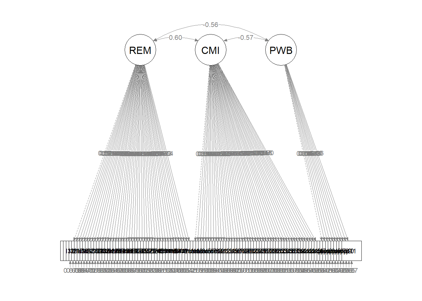
9.8 Interpreting the Output
Now that we’ve had a quick look at the plot, let’s work through the results. Rosseel’s (2019) lavaan tutorial is a useful resource in walking through the output.
The header is the first few lines of the information. It contains:
- the lavaan version number (0.6.16 that I’m using on 10/15/2023),
- maximum likelihood (ML) was used as the estimator,
- confirmation that the specification converged normally after 118 iterations,
- 156 cases were used in this analysis,
9.8.1 Global Fit Indices
CFA falls into a modeling approach to evaluating results. While it provides some flexibility (we get away from the strict, NHST approach of \(p < .05\)) there can be more ambiguity and challenge to interpreting these results. Consequently, researchers will often report a handful of measures that draw from goodness and badness of fit options.
- goodness of fit indices are those where values closer to 1.00 are better
- badness of fit indices are those where values closer to 0.00 are better
9.8.1.1 Model Test User Model:
The chi-square statistic that evaluates the exact-fit hypothesis that there is no difference between the covariances predicted by the model, given the parameter estimates, and the population covariance matrix. Rejecting the hypothesis says that,
- the data contain covariance information that speak against the model, and
- the researcher should explain model-data discrepancies that exceed those expected by sampling error.
Traditional interpretion of the chi-square is an accept-support test where the null hypothesis represents the researchers’ believe that the model is correct. This means that the absence of statistical significance $ (p > .05) $ that supports the model. This is backwards from our usual reject-support test approach. Kline (2016b) recommends that we treat the \(\chi^2\) like a smoke alarm – if the alarm sounds, there may or may not be a fire (a serious model-data discrepancy), but we should treat the alarm seriously and further inspect issues of fit. The \(\chi^2\) is frequently criticized because:
- accept-support test approaches are logically weaker because the failure to disprove an assertion (the exact-fit hypothesis) does not prove that the assertion is true;
- low power (i.e., small sample sizes) makes it more likely that the model will be retained;
- CFA and SEM models require large samples and so the \(\chi^2\) is frequently statistically significant – which rejects the researchers’ model;
For our initial measurement model CFA \(\chi ^{2}(5147)= 7271.391, p < .001\), this significant value is not what we want because it says that our specified model is different than the covariances in the model. At this stage of evaluating the measurement model, this is really critical information. Even though we have freed our latent variables to all covary which each other (which is like the natural state of the covariance matrix to which the model is being compared), the two are statistically significantly different.
9.8.1.2 Model Test Baseline Model
This model is the independence model. That is, there is complete independence of of all variables in the model (i.e., in which all correlations among variables are zero). This is the most restricted model. It is typical for chi-quare values to be quite high (as it is in our example: 13555.967). On its own, this model is not useful to us. It is used, though, in comparisons of incremental fit.
9.8.1.3 Incremental Fit Indices (Located in the User versus Baseline Models section)
Incremental fit indices ask the question, how much better is the fit of our specified model to the data then the baseline model (where it is assumed no relations between the variables). The Comparative Fit Index (CFI) and Tucker-Lewis Index (TLI) are goodness of fit statistics, ranging from 0 to 1.0 where 1.0 is best. Because the two measures are so related, only one should be reported (I typically see the CFI).
CFI: compares the amount of departure from close fit for the researcher’s model against that of the independence/baseline (null) model. When the User and Baseline fits are identical the CFI will equal 1.0. We interpret the value of the CFI as a percent of how much better the researcher’s model is than the baseline model. While 74% sounds like an improvement – Hu and Bentler (1999) stated that “acceptable fit” is achieved when the \(CFI \geq .95\) and \(SRMR \leq .08\); the combination rule. It is important to note that later simulation studies have not supported those thresholds.
TLI: aka the non-normed fit index (NNFI) controls for \(df_M\) from the researcher’s model and \(df_B\) from the baseline model. As such, it imposes a greater relative penalty for model complexity than the CFI. The TLI is a bit unstable in that the values can exceed 1.0.
For our initial measurement model CFA, CFI = 0.744 and TLI = 0.739. While these predict around 74% better than the baseline/independence model, it does not come close to the standard of \(\geq .95\).
9.8.1.4 Loglikelihood and Information Criteria
The Akaike Information Criterion (AIC) and the Bayesian Information Criterion (BIC) utilize an information theory approach to data analysis by combing statistical estimation and model selection into a single framework. The BIC augments the AIC by taking sample size into consideration.
The AIC and BIC are usually used to select among competing nonhierarchical models and are only used in comparison with each other. Thus our current values of 31007.915 (AIC) and 31645.335 (BIC) are meaningless on their own. The model with the smallest value of the predictive fit index is chosen as the one that is most likely to replicate. It means that this model has relatively better fit and fewer free parameters than competing models.
9.8.1.5 Root Mean Square Error of Approximation
The RMSEA is an absolute fit index scaled as a badness-of-fit statistic where a value of 0.00 is the best fit. The RMSEA favors models with more degrees of freedom and larger sample sizes. A unique aspect of the RMSEA is its 90% confidence interval.
While there is chatter/controversy about what constitutes an acceptable value, there is general consensus that \(RMSEA \geq .10\) points to serious problems. An \(RMSEA\leq .05\) is ideal. Watching the upper bound of the confidence interval is important to see that it isn’t sneaking into the danger zone.
For our initial measurement model RMSEA = 0.051, 90% CI(0.049, 0.054). This value is within the accepted thessholds.
9.8.1.6 Standardized Root Mean Square Residual
The SRMR is an absolute fit index that is another badness-of-fit statistic (i.e., perfect model fit is when the value = 0.00 and increasingly higher values indicate the “badness”). The SRMR is a standardized version of the root mean square residual (RMR), which is a measure of the mean absolute covariance residual. Standardizing the value facilitates interpretation. Poor fit is indicated when \(SRMR \geq .10\). For our initial measurement model, SRMR = 0.061. This is within the thressholds of acceptability.
Hu and Bentler (1999) have suggested combination rule (which is somewhat contested) suggested that the SRMR be interpreted along with the CFI such that: \(CFI \geqslant .95\) and \(SRMR \leq .05\). Our initial measurement model does not pass this test: CFI = 0.744, SRMR = 0.061.
9.8.1.7 Factor Loadings
Let’s inspect the latent variables section.
- Estimate contains the estimated or fixed parameter value for each model parameter;
- Std. err is the standard error for each estimated parameter;
- Z-value is the Wald statistic (the parameter divided by its SE)
- P(>|z|) is the p value for testing the null hypothesis that the parameter equals zero in the population
- Std.lv standardizes only the LVs
- Std.all both latent and observed variables are standardized; this is considered the “completely standardized solution”
Note that item Inf32 might seem incomplete – there is only a 1.000 and a value for the Std.lv. Recall that specifying items on a latent variable requires one item to be fixed to 1.000. This “sets the scale” of each latent variable. The default in lavaan::cfa and lavaan::sem is to assign the first of the items used to define the latent variable to this role. Coefficients that are fixed to 1.0 to scale a factor have no standard errors and therefore no significance test. If we looked at the *semPlot::sempath** we can see that arrow line to each of the first indicators per latent variable is different than the others. This is a pictoral representation of setting the scaling on one of the indicator variables.
The SE and associated \(p\) values are associated with the unstandardized estimates. Intuitively, it is easiest for me to understand the relative magnitude of the pattern coefficients by looking at the Std.all column. We can see that the items associated with each of our factors (i.e., REMS, CMI, PWB) are all strong, positive, and statistically significant \((p < 0.001)\) and positive.
9.8.1.8 Adequacy of the Initial Measurement Model
I’ve created a table that allows me to compare our results to the threshholds. I will report the chi-square, CFI, RMSEA, and SRMR. Researchers have different preferences (and different data may be better analyzed by certain indices), so you might find that an editor, professor, or reviewer will ask for something else.
| Criteria | Our Results | Criteria met? |
|---|---|---|
| Factor loadings significant, strong, proper valence | all \(p < 0.001\), lowest = .357(pwb) | Yes |
| Non-significant chi-square | \(\chi ^{2}(5147)= 7271.391, p < .001\) | No |
| \(CFI\geq .95\) (or at least .90) | CFI = 0.744 | No |
| \(RMSEA\leq .05\) (or < .08, at least < .10, also 90CI) | RMSEA = 0.051, 90CI[0.049, 0.054] | Yes |
| \(SRMR\leq .08\) (at least < .10) | SRMR = 0.061 | No |
| Combination rule: \(CFI \geq .95\) & \(SRMR \leq .08\) | CFI = 0.744, SRMR = 0.061 | No |
Our initial measurement model that was defined by all items used as individual indicators for the latent variables and that freed the latent variables to covary had mixed results. While the factor loadins were significant, strong, and properly valanced and the RMSEA and SRMR were within acceptable limits, the chi-square was statistically significant and the CFI was well below 0.95: \(\chi ^{2}(5147)= 7271.391, p < .001, CFI = 0.744, RMSEA = 0.051, 90CI[0.049, 0.054], SRMR = 0.061\). The statistically significant chi-square is not what we want, but also not surprising. While the RMSEA and SRMR are within reasonable limits, the CFI is really substandard.
Concerned about poor model fit associated with the CFI, some researchers might choose to abandon a latent variable approach. After all, the simple mediation we conducted with observed/manifest variables earlier in this text was fine, right? Given the benefits that SEM offers, particularly around the ability to assess measurement error, I suggest that it is worth our time to consider the contribution of parceling to see if we can improve the fit of our measurement model.
9.9 Parceling
In the context of SEM, parceling can reduce the complexity in latent variables by creating composites or parcels of observed variables. For latent variables with numerous indicators, parceling can be an option that simplifies the model and can improve fit. A parcel is an aggregate-level indicator comprised of the sum (or average) of two or more items, responses, or behaviors. Parcels represent the manifest (observed) variables.
Little et al. (2002) outlined the pros and cons of parceling and provided a practical guidelines for doing so. Although parceling has become more common place, it remains controversial. Kline (2016b) is not a huge fan (see pp. 331-332) and Byrne (Byrne, 2016a) merely provided a general description of the process without demonstrating it in the examples wshe provided. Little, remains a proponent and has updated the rationale and circumstances when parceling is appropriate (T. D. Little et al., 2013).
9.9.1 The Pros and Cons of Parceling
The Little et al. (2002) article reviewed the rather heated arguments for and against parcels on from three perspectives: philosophical, psychometric, modelers. Below I highlight each.
9.9.1.1 Philosophical Arguments
Empiricist-conservativists claim that modeled data should be (or be as close to possible) as the original individual responses of the research participants. Re-modeling data risks mis-representation and could be considered to be “cheating.” Further, they claim that parceling items “fundamentally undermines the objective empirical purpose of the techniques that have been developed to model multivariate data” (Little et al., 2002, p. 152).
Pragmatic-liberals suggest that representing each and every source of variance for each item is impossible. At best, we hope that our models represent the important common sources of variance across samples of items. Consequently, our goal is to build replicable models based on stable, meaningful indicators of core constructs. Correspondingly, pragmatic-liberals suggest that using parcels as the lowest level of data to be modeled is acceptable if the research project utilized a strict, rule-bound system of data collection and reporting. Further, it is essential for the researcher to describe what they have done and provide a rationale for doing so. As always, editors/reviewers have the right to reject the work and subsequent researchers can refute it.
9.9.1.2 Psychometric Arguments
Psychometricians point out that, compared to parcels, items have fewer, larger, and less equal intervals between scale points. Consequently, models built on item-level data tend to have lower reliability, lower communality, smaller ratio of common-to-unique factor variance, and increased likelihood of distributional violations. Additionally, because parcels permit factors to be defined with fewer constructs, they are preferred – especially when sample size is an issue. In short, models built on parceled data:
- Are more parsimonious (i.e., have fewer estimated parameters)
- Have fewer chances for residuals to be correlated or cross-loadings (b/c fewer indicators are needed and unique variances are smaller)
- Lead to reductions in various sources of sampling error
- Provide greater representation of the construct because aggregate scores are used
- Provide a more consistent and reliable representation of the construct because aggregate scores are used
- Reduce the problems associated when latent variables have a large number of indicators
Psychomtricians do offer one significant caution – parceling should only be used with unidimensional constructs and not with multidimensional ones. Practically, this could mean that the latent variable has a confirmatory factor analysis that supports a unidimensional, second order, or g scale in a bifactor structure. If unidimensionality is uncertain, preliminary psychometric evaluation could be in order.There seems to be some controversy about “how unidimensional” it should be. Little (2013) seems to acknowledge that multidimensional instruments are sometimes used.
Further, parceling is completely inappropriate when establishing the psychometric properties of an instrument. The use of parceling should be reserved for utilizing that instrument to testa theoretical model.
9.9.1.3 Modelers’ Arguments
Modeling at the item level increases the likelihood that subsets of items will share specific sources of variance (which, themselves, represent latent variables). Because they are unlikely to be hypothesized by the researcher, they will lead to systematic sources of common variance that were not specified a priori. In contrast, parceling eliminates or at least reduces unwanted sources of variance and leads to better initial model fit and reduces the likelihood of misspecification. Further, because parceling improves the psychometric characteristics of items, solutions are more stable (i.e., requiring more iterations to converge, yielding relatively large standard errors of the measurement model, poorer fit).
Modelers have pointed out that item-level modeling inflates Type I error. Here’s how:
- If we assume that 5% of all correlations are error (p < .05), a model with 3 constructs – each measured with 10 variables – would result in 22 spurious correlations.
- In contrast, a structural model with 3 constructs, each measured with 3 parcels each, would yield ~ 2 spurious correlations. The nature of which would be evidenced with a failure to replicate.
Modelers do point out issues related to model identification. Representing a latent variable with one or two items is possible, but is suboptimal because the latent variable is underidentified. A just-identified latent contains 3 indicators; 4 or more leads to an overidentified latent variable. In arguments made more than a decade after the 2002 article, Little and colleagues (2013) recommend using 3 indicators (which could be parcels) per construct.
Modelers who caution against modeling suggest that parcel-based models attempt to cancel out random and systematic error by aggregrating across these errors. While the typical improvement in model fit is desirable, some argue is that it changes the reality of the data, and therefore misrepresents it. In-so-doing, it can hide mis-specification of the model. Some have argued that parceling should be reserved for theoretical work and is probably not appropriate for applied work when norms based on established measures are used.
9.9.2 Practical Procedures for Parceling
There are several approaches to creating parcels. Byrne (2016a) distinguished between purposive and random approaches to parceling.
9.9.2.1 Purposive Approaches to Parceling
Utilizing subscale scores as parcels is, perhaps, the most common (and intuitively appealing) example of a purposive approach to parceling. This approach can be appropriate in certain circumstances if (a) it is theoretically justified and (b) if the psychometric properties of the scales are sound. This approach can be problematic if (a) the factor loadings of the subscales are unequal and/or (b) if there aren’t at least three subscales. While it is possible to have a factor with just two loadings, these are more likely to havce improper solutions such as Heywood cases.
The item-to-construct balance is another purposive approach. The goal is to derive parcels that are equally balanced in terms of difficulty and discrimination (i.e., intercept and slope). If the researcher were creating a latent variable with three parcels (i.e., three indicators), the researcher would obtain and rank order the factor loadings. The three items with the highest loadings would be assigned to the three parcels first (let’s call them A, B, C), the next three highest loadings would be added to the parcels in a reversed order (C, B, A), the next three reversed again (A, B, C), continuing back and forth until all items are assigned. In some conditions, parcels may have differential numbers of items in order to achieve a reasonable balance.
9.9.2.2 Random Approaches to Parceling
Random assignment is, perhaps, the most common way that parcels are created. Little et al. (2013) has recommended that each construct in an SEM model should be just-identified with three indicators per construct. Because this provides a precise definition of the construct, it is seen to be a super test. Thus, who engage in this practice will assign indicators, randomly (without replacement) to th three parcels. The result should be parcels with roughly equal common factor variance.
To illustrate the similarities and differences between approaches, I will evaluate two measurement models: one by using subscale scores and another with random assignment to three parcels per construct.
9.10 Parceling with Subscale Scores
Parceling with subscale scores means that you simply include the items that belong to each subscale in a parcel. Thus, it is often necessary to consult the journal articles and/or test manuals that provide information about the instrument. When simulating the data from the journal article, I was able to retrieve information about the psychometric development and evaluation of the REMS (Nadal, 2011), but not the CMI (Terrell & Terrell, 1981) or the MHI/PwB (Veit & Ware, 1983). Thus, in working the subscale example, I will make some incorrect assumptions about the relations between the items and measures.
The 45 items of the REMS are divided between six subscales; thus, parceling by subscale will result in six indicators for the REMS factor. In simulating the data, I was able to use the factor loadings from each item as it relates to each scale. To facilitate subsequent analyses, I provided abbreviations of the scale names. Practically speaking, creating parcels is to score the subscales. In the script below, I create first create concatonated lists of the variables. Second, I calculate mean scores if 80% of the items for each respondent are non-missing. You may recognize this as being consistent with Parent’s (2013) available information analysis (AIA) approach to managing missingness. I have written more on the AIA approach in a lesson on Scoring data.
Inf_vars <- c("Inf32", "Inf38", "Inf21", "Inf17", "Inf9", "Inf36", "Inf5",
    "Inf22")
SClass_vars <- c("SClass8", "SClass40", "SClass2", "SClass34", "SClass11")
mInv_vars <- c("mInv27", "mInv39", "mInv7", "mInv26", "mInv33", "mInv4",
    "mInv14", "mInv10")
Exot_vars <- c("Exot3", "Exot29", "Exot45", "Exot35", "Exot42", "Exot23",
    "Exot13", "Exot20", "Exot43")
mEnv_vars <- c("mEnv37", "mEnv24", "mEnv19", "mEnv28", "mEnv18", "mEnv41",
    "mEnv12")
mWork_vars <- c("mWork25", "mWork15", "mWork1", "mWork16", "mWork44")

dfKim$Inf_P <- sjstats::mean_n(dfKim[, Inf_vars], 0.8)
dfKim$SClass_P <- sjstats::mean_n(dfKim[, SClass_vars], 0.8)
dfKim$mInv_P <- sjstats::mean_n(dfKim[, mInv_vars], 0.8)
dfKim$Exot_P <- sjstats::mean_n(dfKim[, Exot_vars], 0.8)
dfKim$mEnv_P <- sjstats::mean_n(dfKim[, mEnv_vars], 0.8)
dfKim$mWork_P <- sjstats::mean_n(dfKim[, mWork_vars], 0.8)

# If the scoring code above does not work for you, try the format
# below which involves inserting to periods in front of the variable
# list. One example is provided. dfKim$mWork_P <-
# sjstats::mean_n(dfKim[,.. mWork_vars], .80)
We learn from Kim et al’s description (Paul Youngbin Kim et al., 2017) that the CMI has four factors. Because I could not retrieve an article with original psychometrics, I was not able to provide factor correlations and my variable names do not reflect scale membership. Let’s pretend that the items are in order of the scales. i will assign 12 items each to the first three scales and 11 items to the fourth scale.
IntRel_vars <- c("cmi1", "cmi2", "cmi3", "cmi4", "cmi5", "cmi6", "cmi7",
    "cmi8", "cmi9", "cmi10", "cmi11", "cmi12")
EdTrain_vars <- c("cmi13", "cmi14", "cmi15", "cmi16", "cmi17", "cmi18",
    "cmi19", "cmi20", "cmi21", "cmi22", "cmi23", "cmi24")
BusWrk_vars <- c("cmi25", "cmi26", "cmi27", "cmi28", "cmi29", "cmi30",
    "cmi31", "cmi32", "cmi33", "cmi34", "cmi35", "cmi36")
PolLaw_vars <- c("cmi37", "cmi38", "cmi39", "cmi40", "cmi41", "cmi42",
    "cmi43", "cmi44", "cmi45", "cmi46", "cmi47")

dfKim$IntRel <- sjstats::mean_n(dfKim[, IntRel_vars], 0.8)
dfKim$EdTrain <- sjstats::mean_n(dfKim[, EdTrain_vars], 0.8)
dfKim$BusWrk <- sjstats::mean_n(dfKim[, BusWrk_vars], 0.8)
dfKim$PolLaw <- sjstats::mean_n(dfKim[, PolLaw_vars], 0.8)

# If the scoring code above does not work for you, try the format
# below which involves inserting to periods in front of the variable
# list. One example is provided. dfKim$PolLaw <-
# sjstats::mean_n(dfKim[, ..PolLaw_vars], .80)
The description of the MHI only indicates that there are items on the PWB scale (and not that there are further subscales). This gives us some choice about how to divide the items. I would likely be inclined to randomly divide them across three scales.
The following code will provide random assignments.
set.seed(230916)
items <- c("pwb1", "pwb2", "pwb3", "pwb4", "pwb5", "pwb6", "pwb7", "pwb8",
    "pwb9", "pwb10", "pwb11")
parcels <- c("PWB_p1", "PWB_p_2", "PWB_p3")
data.frame(items = sample(items), parcel = rep(parcels, length = length(items)))
## items parcel
## 1 pwb7 PWB_p1
## 2 pwb9 PWB_p_2
## 3 pwb1 PWB_p3
## 4 pwb11 PWB_p1
## 5 pwb2 PWB_p_2
## 6 pwb3 PWB_p3
## 7 pwb4 PWB_p1
## 8 pwb10 PWB_p_2
## 9 pwb5 PWB_p3
## 10 pwb8 PWB_p1
## 11 pwb6 PWB_p_2We can now create the parcels using the same scoring procedure as we did for the REMS and CMI instruments.
PWB_p1_vars <- c("pwb7", "pwb11", "pwb4", "pwb8")
PWB_p2_vars <- c("pwb9", "pwb2", "pwb10", "pwb2")
PWB_p3_vars <- c("pwb1", "pwb3", "pwb5")

dfKim$p1PWB <- sjstats::mean_n(dfKim[, PWB_p1_vars], 0.75)
dfKim$p2PWB <- sjstats::mean_n(dfKim[, PWB_p2_vars], 0.75)
dfKim$p3PWB <- sjstats::mean_n(dfKim[, PWB_p3_vars], 0.75)

# If the scoring code above does not work for you, try the format
# below which involves inserting to periods in front of the variable
# list. One example is provided. dfKim$p3PWB <-
# sjstats::mean_n(dfKim[, ..PWB_p3_vars], .75)
Before we continue to respecifying the measurement model, let me point out that a downside of using subscales as parcels is that it Little et al’s (2013) recommendation is that each latent variable be represented with a just-identified (i.e., 3-parcel) solution. Like our circumstance where the REMS has six subscales and the CMI has four, it is frequently the case where measures have differing numbers of solutions. When there are more than three parcels, the fit of the measurement model is likely to be worse than if there were three parcels per latent variable.
9.10.1 Measurement Model with Subscale Parcels
Let’s respecify our measurement model with parcels created from subscale means.
subsc_msmt_mod <- "
        ##measurement model
         REMS =~ Inf_P + SClass_P + mInv_P + Exot_P + mEnv_P + mWork_P

         CMI =~ IntRel + EdTrain + BusWrk + PolLaw

         PWB =~ p1PWB + p2PWB + p3PWB


        # Covariances
         REMS ~~ CMI
         REMS ~~ PWB
         CMI ~~ PWB
        "

set.seed(230916)
subsc_msmt_fit <- lavaan::cfa(subsc_msmt_mod, data = dfKim, missing = "fiml")
# , missing = 'fiml' #deleted this from the above code because it
# seemed to be slowing it down
subsc_msmt_fit_sum <- lavaan::summary(subsc_msmt_fit, fit.measures = TRUE,
    standardized = TRUE)
subsc_msmt_fit_sum
## lavaan 0.6.17 ended normally after 127 iterations
##
## Estimator ML
## Optimization method NLMINB
## Number of model parameters 42
##
## Number of observations 156
## Number of missing patterns 1
##
## Model Test User Model:
##
## Test statistic 71.488
## Degrees of freedom 62
## P-value (Chi-square) 0.192
##
## Model Test Baseline Model:
##
## Test statistic 2095.199
## Degrees of freedom 78
## P-value 0.000
##
## User Model versus Baseline Model:
##
## Comparative Fit Index (CFI) 0.995
## Tucker-Lewis Index (TLI) 0.994
##
## Robust Comparative Fit Index (CFI) 0.995
## Robust Tucker-Lewis Index (TLI) 0.994
##
## Loglikelihood and Information Criteria:
##
## Loglikelihood user model (H0) -379.365
## Loglikelihood unrestricted model (H1) -343.621
##
## Akaike (AIC) 842.731
## Bayesian (BIC) 970.825
## Sample-size adjusted Bayesian (SABIC) 837.881
##
## Root Mean Square Error of Approximation:
##
## RMSEA 0.031
## 90 Percent confidence interval - lower 0.000
## 90 Percent confidence interval - upper 0.060
## P-value H_0: RMSEA <= 0.050 0.839
## P-value H_0: RMSEA >= 0.080 0.001
##
## Robust RMSEA 0.031
## 90 Percent confidence interval - lower 0.000
## 90 Percent confidence interval - upper 0.060
## P-value H_0: Robust RMSEA <= 0.050 0.839
## P-value H_0: Robust RMSEA >= 0.080 0.001
##
## Standardized Root Mean Square Residual:
##
## SRMR 0.024
##
## Parameter Estimates:
##
## Standard errors Standard
## Information Observed
## Observed information based on Hessian
##
## Latent Variables:
## Estimate Std.Err z-value P(>|z|) Std.lv Std.all
## REMS =~
## Inf_P 1.000 0.275 0.884
## SClass_P 0.980 0.062 15.722 0.000 0.270 0.873
## mInv_P 0.993 0.063 15.852 0.000 0.273 0.878
## Exot_P 0.986 0.058 17.018 0.000 0.271 0.907
## mEnv_P 1.073 0.063 17.131 0.000 0.295 0.903
## mWork_P 1.066 0.069 15.337 0.000 0.293 0.864
## CMI =~
## IntRel 1.000 0.760 0.948
## EdTrain 0.972 0.040 24.289 0.000 0.739 0.939
## BusWrk 0.974 0.040 24.475 0.000 0.740 0.939
## PolLaw 1.056 0.040 26.144 0.000 0.802 0.953
## PWB =~
## p1PWB 1.000 0.305 0.634
## p2PWB 1.610 0.229 7.044 0.000 0.492 0.802
## p3PWB 1.373 0.206 6.654 0.000 0.419 0.708
##
## Covariances:
## Estimate Std.Err z-value P(>|z|) Std.lv Std.all
## REMS ~~
## CMI 0.126 0.021 6.024 0.000 0.604 0.604
## PWB -0.047 0.010 -4.615 0.000 -0.554 -0.554
## CMI ~~
## PWB -0.130 0.027 -4.753 0.000 -0.560 -0.560
##
## Intercepts:
## Estimate Std.Err z-value P(>|z|) Std.lv Std.all
## .Inf_P 0.502 0.025 20.145 0.000 0.502 1.613
## .SClass_P 0.485 0.025 19.596 0.000 0.485 1.569
## .mInv_P 0.523 0.025 21.003 0.000 0.523 1.682
## .Exot_P 0.508 0.024 21.218 0.000 0.508 1.699
## .mEnv_P 0.504 0.026 19.255 0.000 0.504 1.542
## .mWork_P 0.462 0.027 16.985 0.000 0.462 1.360
## .IntRel 4.030 0.064 62.745 0.000 4.030 5.024
## .EdTrain 3.824 0.063 60.645 0.000 3.824 4.855
## .BusWrk 3.907 0.063 61.872 0.000 3.907 4.954
## .PolLaw 4.003 0.067 59.382 0.000 4.003 4.754
## .p1PWB 3.014 0.039 78.207 0.000 3.014 6.262
## .p2PWB 3.207 0.049 65.324 0.000 3.207 5.230
## .p3PWB 3.141 0.047 66.276 0.000 3.141 5.306
##
## Variances:
## Estimate Std.Err z-value P(>|z|) Std.lv Std.all
## .Inf_P 0.021 0.003 7.367 0.000 0.021 0.219
## .SClass_P 0.023 0.003 7.567 0.000 0.023 0.238
## .mInv_P 0.022 0.003 7.505 0.000 0.022 0.230
## .Exot_P 0.016 0.002 6.921 0.000 0.016 0.177
## .mEnv_P 0.020 0.003 7.002 0.000 0.020 0.184
## .mWork_P 0.029 0.004 7.651 0.000 0.029 0.254
## .IntRel 0.066 0.010 6.438 0.000 0.066 0.102
## .EdTrain 0.074 0.011 6.821 0.000 0.074 0.119
## .BusWrk 0.074 0.011 6.790 0.000 0.074 0.118
## .PolLaw 0.065 0.011 6.126 0.000 0.065 0.092
## .p1PWB 0.139 0.019 7.313 0.000 0.139 0.598
## .p2PWB 0.134 0.029 4.615 0.000 0.134 0.357
## .p3PWB 0.175 0.028 6.316 0.000 0.175 0.498
## REMS 0.076 0.011 6.991 0.000 1.000 1.000
## CMI 0.578 0.073 7.935 0.000 1.000 1.000
## PWB 0.093 0.024 3.957 0.000 1.000 1.000As we look at the results we can easily see the benefits to the model. The factor loadings are strong, significant, and all scoring in the correct (positive) direction. The fit indices are much improved. Let’s take a look according to the criteria we are using:
| Criteria | Our Results | Criteria met? |
|---|---|---|
| Factor loadings significant, strong, proper valence | all \(p < 0.001\), lowest = .634(pwb) | Yes |
| Non-significant chi-square | \(\chi ^{2}(62)= 71.488, p = 0.192\) | Yes |
| \(CFI\geq .95\) (or at least .90) | CFI = 0.995 | Yes |
| \(RMSEA\leq .05\) (or < .08, at least < .10, also 90CI) | RMSEA = 0.031, 90CI[0.000, 0.060] | Yes |
| \(SRMR\leq .08\) (at least < .10) | SRMR = 0.024 | Yes |
| Combination rule: \(CFI \geq .95\) & \(SRMR \leq .08\) | CFI = 0.995, SRMR = 0.024 | Yes |
The measurement model created by parcels that represent subscales of the instruments (i.e., defined by prior psychometric evaluation) has dramatically improved. The chi-square is no longer statistically significant and the CFI is > 0.95: \(\chi^2(62) = 71.488, p = 0.192, CFI = 0.995, RMSEA = 0.031, 90CI[0.000, 0.060], SRMR = 0.024\). This might be a sufficient solution. An option that is more consistent with Little et al’s (T. D. Little et al., 2013) recommendation for factors that are just-identified, is one that is constructed randomly.
9.10.2 Measurement Model with Just-Identified Random Parcels
In the prior example, we created three parcels through random assignment for the PWB scale. We can use those same parcels. We repeat those steps for the REMS and CMI scales. This code randomly assigns the 45 REMS items across the three parcels.
set.seed(230916)
items <- c("Inf32", "Inf38", "Inf21", "Inf17", "Inf9", "Inf36", "Inf5",
    "Inf22", "SClass6", "SClass31", "SClass8", "SClass40", "SClass2", "SClass34",
    "SClass11", "mInv27", "mInv30", "mInv39", "mInv7", "mInv26", "mInv33",
    "mInv4", "mInv14", "mInv10", "Exot3", "Exot29", "Exot45", "Exot35",
    "Exot42", "Exot23", "Exot13", "Exot20", "Exot43", "mEnv37", "mEnv24",
    "mEnv19", "mEnv28", "mEnv18", "mEnv41", "mEnv12", "mWork25", "mWork15",
    "mWork1", "mWork16", "mWork44")
parcels <- c("REMS_p1", "REMS_p2", "REMS_p3")
data.frame(items = sample(items), parcel = rep(parcels, length = length(items)))
## items parcel
## 1 mWork44 REMS_p1
## 2 mEnv41 REMS_p2
## 3 mWork25 REMS_p3
## 4 Exot20 REMS_p1
## 5 SClass11 REMS_p2
## 6 Inf38 REMS_p3
## 7 SClass8 REMS_p1
## 8 Inf5 REMS_p2
## 9 Inf17 REMS_p3
## 10 Exot43 REMS_p1
## 11 mEnv19 REMS_p2
## 12 Exot23 REMS_p3
## 13 mInv4 REMS_p1
## 14 mInv39 REMS_p2
## 15 mInv33 REMS_p3
## 16 SClass31 REMS_p1
## 17 Inf22 REMS_p2
## 18 mEnv28 REMS_p3
## 19 SClass40 REMS_p1
## 20 mEnv18 REMS_p2
## 21 Inf36 REMS_p3
## 22 mWork16 REMS_p1
## 23 mInv30 REMS_p2
## 24 mInv14 REMS_p3
## 25 Exot45 REMS_p1
## 26 Inf32 REMS_p2
## 27 mEnv37 REMS_p3
## 28 SClass2 REMS_p1
## 29 SClass34 REMS_p2
## 30 Inf21 REMS_p3
## 31 Exot3 REMS_p1
## 32 Exot29 REMS_p2
## 33 mEnv12 REMS_p3
## 34 mEnv24 REMS_p1
## 35 mInv27 REMS_p2
## 36 Exot42 REMS_p3
## 37 Exot35 REMS_p1
## 38 mInv10 REMS_p2
## 39 SClass6 REMS_p3
## 40 mInv7 REMS_p1
## 41 mWork1 REMS_p2
## 42 Inf9 REMS_p3
## 43 Exot13 REMS_p1
## 44 mWork15 REMS_p2
## 45 mInv26 REMS_p3This code provides means for each of the three REMS parcels.
REMS_p1_vars <- c("mWork44", "Exot20", "SClass8", "Exot43", "mInv4", "SClass31",
    "SClass40", "mWork16", "Exot45", "SClass2", "Exot3", "mEnv24", "Exot35",
    "mInv7", "Exot13")
REMS_p2_vars <- c("mEnv41", "SClass11", "Inf5", "mEnv19", "mInv39", "Inf22",
    "mEnv18", "mInv30", "Inf32", "SClass34", "Exot29", "mInv27", "mInv10",
    "mWork1", "mWork15")
REMS_p3_vars <- c("mWork25", "Inf38", "Inf17", "Exot23", "mInv33", "mEnv28",
    "Inf36", "mInv14", "mEnv37", "Inf21", "mEnv12", "Exot42", "SClass6",
    "Inf9", "mInv26")

dfKim$p1REMS <- sjstats::mean_n(dfKim[, REMS_p1_vars], 0.8)
dfKim$p2REMS <- sjstats::mean_n(dfKim[, REMS_p2_vars], 0.8)
dfKim$p3REMS <- sjstats::mean_n(dfKim[, REMS_p3_vars], 0.8)

# If the scoring code above does not work for you, try the format
# below which involves inserting to periods in front of the variable
# list. One example is provided. dfKim$p3REMS <-
# sjstats::mean_n(dfKim[, ..REMS_p3_vars], .80)
We can repeat the process for the CMI. First, we assign the 47 CMI items to the three parcels.
set.seed(230916)
items <- c(IntRel_vars <- c("cmi1", "cmi2", "cmi3", "cmi4", "cmi5", "cmi6",
    "cmi7", "cmi8", "cmi9", "cmi10", "cmi11", "cmi12", "cmi13", "cmi14",
    "cmi15", "cmi16", "cmi17", "cmi18", "cmi19", "cmi20", "cmi21", "cmi22",
    "cmi23", "cmi24", "cmi25", "cmi26", "cmi27", "cmi28", "cmi29", "cmi30",
    "cmi31", "cmi32", "cmi33", "cmi34", "cmi35", "cmi36", "cmi37", "cmi38",
    "cmi39", "cmi40", "cmi41", "cmi42", "cmi43", "cmi44", "cmi45", "cmi46",
    "cmi47"))
parcels <- c("CMI_p1", "CMI_p2", "CMI_p3")
data.frame(items = sample(items), parcel = rep(parcels, length = length(items)))
## items parcel
## 1 cmi45 CMI_p1
## 2 cmi39 CMI_p2
## 3 cmi41 CMI_p3
## 4 cmi32 CMI_p1
## 5 cmi15 CMI_p2
## 6 cmi2 CMI_p3
## 7 cmi11 CMI_p1
## 8 cmi7 CMI_p2
## 9 cmi4 CMI_p3
## 10 cmi33 CMI_p1
## 11 cmi38 CMI_p2
## 12 cmi30 CMI_p3
## 13 cmi22 CMI_p1
## 14 cmi18 CMI_p2
## 15 cmi46 CMI_p3
## 16 cmi12 CMI_p1
## 17 cmi40 CMI_p2
## 18 cmi6 CMI_p3
## 19 cmi26 CMI_p1
## 20 cmi47 CMI_p2
## 21 cmi17 CMI_p3
## 22 cmi25 CMI_p1
## 23 cmi27 CMI_p2
## 24 cmi23 CMI_p3
## 25 cmi44 CMI_p1
## 26 cmi1 CMI_p2
## 27 cmi10 CMI_p3
## 28 cmi13 CMI_p1
## 29 cmi14 CMI_p2
## 30 cmi3 CMI_p3
## 31 cmi31 CMI_p1
## 32 cmi42 CMI_p2
## 33 cmi29 CMI_p3
## 34 cmi34 CMI_p1
## 35 cmi8 CMI_p2
## 36 cmi28 CMI_p3
## 37 cmi37 CMI_p1
## 38 cmi19 CMI_p2
## 39 cmi21 CMI_p3
## 40 cmi43 CMI_p1
## 41 cmi20 CMI_p2
## 42 cmi35 CMI_p3
## 43 cmi24 CMI_p1
## 44 cmi5 CMI_p2
## 45 cmi36 CMI_p3
## 46 cmi9 CMI_p1
## 47 cmi16 CMI_p2This code provides means for each of the three CMI parcels.
CMI_p1_vars <- c("cmi45", "cmi32", "cmi11", "cmi33", "cmi22", "cmi12",
    "cmi26", "cmi25", "cmi44", "cmi13", "cmi31", "cmi34", "cmi37", "cmi43",
    "cmi24", "cmi9")
CMI_p2_vars <- c("cmi39", "cmi15", "cmi7", "cmi38", "cmi18", "cmi40", "cmi47",
    "cmi27", "cmi1", "cmi14", "cmi42", "cmi8", "cmi19", "cmi20", "cmi5",
    "cmi16")
CMI_p3_vars <- c("cmi41", "cmi2", "cmi4", "cmi30", "cmi46", "cmi6", "cmi17",
    "cmi23", "cmi10", "cmi3", "cmi29", "cmi28", "cmi21", "cmi35", "cmi36")

dfKim$p1CMI <- sjstats::mean_n(dfKim[, CMI_p1_vars], 0.8)
dfKim$p2CMI <- sjstats::mean_n(dfKim[, CMI_p2_vars], 0.8)
dfKim$p3CMI <- sjstats::mean_n(dfKim[, CMI_p3_vars], 0.8)

# If the scoring code above does not work for you, try the format
# below which involves inserting to periods in front of the variable
# list. One example is provided. dfKim$p3CMI <-
# sjstats::mean_n(dfKim[, ..CMI_p3_vars], .80)
9.10.2.1 Evaluating the Randomly Identified Measurement Model
We can now evaluate the measurement model that is defined by each scale’s items that were randomly assigned to three parcels, each.
rp3_msmt_mod <- "
        ##measurement model
         REMS =~ p1REMS + p2REMS + p3REMS

         CMI =~ p1CMI + p2CMI + p3CMI

         PWB =~ p1PWB + p2PWB + p3PWB


        # Covariances
         REMS ~~ CMI
         REMS ~~ PWB
         CMI ~~ PWB
        "

set.seed(230916)
rp3_msmt_fit <- lavaan::cfa(rp3_msmt_mod, data = dfKim, missing = "fiml")
rp3_msmt_fit_sum <- lavaan::summary(rp3_msmt_fit, fit.measures = TRUE,
    standardized = TRUE)
rp3_msmt_fit_sum
## lavaan 0.6.17 ended normally after 106 iterations
##
## Estimator ML
## Optimization method NLMINB
## Number of model parameters 30
##
## Number of observations 156
## Number of missing patterns 1
##
## Model Test User Model:
##
## Test statistic 15.965
## Degrees of freedom 24
## P-value (Chi-square) 0.889
##
## Model Test Baseline Model:
##
## Test statistic 1366.804
## Degrees of freedom 36
## P-value 0.000
##
## User Model versus Baseline Model:
##
## Comparative Fit Index (CFI) 1.000
## Tucker-Lewis Index (TLI) 1.009
##
## Robust Comparative Fit Index (CFI) 1.000
## Robust Tucker-Lewis Index (TLI) 1.009
##
## Loglikelihood and Information Criteria:
##
## Loglikelihood user model (H0) -368.149
## Loglikelihood unrestricted model (H1) -360.166
##
## Akaike (AIC) 796.297
## Bayesian (BIC) 887.793
## Sample-size adjusted Bayesian (SABIC) 792.834
##
## Root Mean Square Error of Approximation:
##
## RMSEA 0.000
## 90 Percent confidence interval - lower 0.000
## 90 Percent confidence interval - upper 0.031
## P-value H_0: RMSEA <= 0.050 0.988
## P-value H_0: RMSEA >= 0.080 0.000
##
## Robust RMSEA 0.000
## 90 Percent confidence interval - lower 0.000
## 90 Percent confidence interval - upper 0.031
## P-value H_0: Robust RMSEA <= 0.050 0.988
## P-value H_0: Robust RMSEA >= 0.080 0.000
##
## Standardized Root Mean Square Residual:
##
## SRMR 0.017
##
## Parameter Estimates:
##
## Standard errors Standard
## Information Observed
## Observed information based on Hessian
##
## Latent Variables:
## Estimate Std.Err z-value P(>|z|) Std.lv Std.all
## REMS =~
## p1REMS 1.000 0.271 0.944
## p2REMS 1.055 0.044 23.770 0.000 0.286 0.946
## p3REMS 1.031 0.046 22.399 0.000 0.280 0.929
## CMI =~
## p1CMI 1.000 0.773 0.963
## p2CMI 1.006 0.035 28.780 0.000 0.778 0.957
## p3CMI 0.937 0.034 27.373 0.000 0.724 0.948
## PWB =~
## p1PWB 1.000 0.306 0.635
## p2PWB 1.606 0.228 7.055 0.000 0.491 0.801
## p3PWB 1.372 0.206 6.662 0.000 0.420 0.709
##
## Covariances:
## Estimate Std.Err z-value P(>|z|) Std.lv Std.all
## REMS ~~
## CMI 0.128 0.021 6.199 0.000 0.608 0.608
## PWB -0.047 0.010 -4.712 0.000 -0.562 -0.562
## CMI ~~
## PWB -0.132 0.028 -4.763 0.000 -0.559 -0.559
##
## Intercepts:
## Estimate Std.Err z-value P(>|z|) Std.lv Std.all
## .p1REMS 0.494 0.023 21.448 0.000 0.494 1.717
## .p2REMS 0.504 0.024 20.790 0.000 0.504 1.665
## .p3REMS 0.522 0.024 21.642 0.000 0.522 1.733
## .p1CMI 3.888 0.064 60.479 0.000 3.888 4.842
## .p2CMI 3.886 0.065 59.667 0.000 3.886 4.777
## .p3CMI 4.051 0.061 66.190 0.000 4.051 5.299
## .p1PWB 3.014 0.039 78.207 0.000 3.014 6.262
## .p2PWB 3.207 0.049 65.324 0.000 3.207 5.230
## .p3PWB 3.141 0.047 66.276 0.000 3.141 5.306
##
## Variances:
## Estimate Std.Err z-value P(>|z|) Std.lv Std.all
## .p1REMS 0.009 0.002 5.466 0.000 0.009 0.109
## .p2REMS 0.010 0.002 5.330 0.000 0.010 0.106
## .p3REMS 0.012 0.002 6.278 0.000 0.012 0.137
## .p1CMI 0.047 0.009 5.046 0.000 0.047 0.072
## .p2CMI 0.056 0.010 5.597 0.000 0.056 0.084
## .p3CMI 0.060 0.009 6.292 0.000 0.060 0.102
## .p1PWB 0.138 0.019 7.309 0.000 0.138 0.597
## .p2PWB 0.135 0.029 4.646 0.000 0.135 0.358
## .p3PWB 0.174 0.028 6.320 0.000 0.174 0.498
## REMS 0.074 0.009 7.838 0.000 1.000 1.000
## CMI 0.598 0.073 8.171 0.000 1.000 1.000
## PWB 0.093 0.024 3.963 0.000 1.000 1.000How do the results of the measurement model created by three parcels, created by random assignment of indicators to each, fare?
| Criteria | Our Results | Criteria met? |
|---|---|---|
| Factor loadings significant, strong, proper valence | all \(p < 0.001\), lowest = .635(pwb) | Yes |
| Non-significant chi-square | \(\chi ^{2}(24) = 15.965, p = 0.889\) | Yes |
| \(CFI\geq .95\) (or at least .90) | CFI = 1.000 | Yes |
| \(RMSEA\leq .05\) (or < .08, at least < .10, also 90CI) | RMSEA = 0.000, 90CI[0.000, 0.031] | Yes |
| \(SRMR\leq .08\) (at least < .10) | SRMR = 0.017 | Yes |
| Combination rule: \(CFI \geq .95\) & \(SRMR \leq .08\) | CFI = 1.000, SRMR = 0.017 | Yes |
The measurement model created by three parcels, created by random assignment of indicators to each has improved, even further: \(\chi^2(24) = 15.965, p = 0.889, CFI = 1.000, RMSEA = 0.000, 90CI[0.000, 0.031], SRMR = 0.017\)
Results of the evaluation of the measurement model can be exported as .csv files with the following code. These produce output that include global fit indices, parameter estimates, and correlations between the latent variables, respectively. The tidySEM::table_fit function will display all of the global fit indices.
# global fit indices
rp3_msmt_fitstats <- tidySEM::table_fit(rp3_msmt_fit)
write.csv(rp3_msmt_fitstats, file = "rp3_msmt_fitstats.csv")
# parameter estimates
rp3_msmt_pEsts <- tidySEM::table_results(rp3_msmt_fit, digits = 3, columns = NULL)
write.csv(rp3_msmt_pEsts, file = "rp3_msmt_pEsts.csv")
# correlations between latent variables
rp3_msmt_LVcorr <- tidySEM::table_cors(rp3_msmt_fit, digits = 3)
write.csv(rp3_msmt_LVcorr, file = "rp3_msmt_LVcorr.csv")
The diagramming function semPlot::semPaths can make a pretty good “guess” at simple models such as these. Given that it is unlikely that there would be room for displaying the measurement model in a journal article, there is generally no need to tinker with it too much.
semPlot::semPaths(rp3_msmt_fit, what = "col", whatLabels = "stand", sizeMan = 5,
    node.width = 1, edge.label.cex = 0.75, style = "lisrel", mar = c(5,
        5, 5, 5))
9.10.3 APA Style Write-up of the Results
Earlier in its history, researchers would spend considerable time describing their measurement model and, if they had used it, defending their use of parceling. One of my favorite write-ups occurs in Mallinckrodt et al.’s 2005 article(2005). Because it is one of the most complete descriptions I have seen, I have consulted it again and again as I have made decisions about my own models. More recent articles describe (Autin et al., 2022; Tokar et al., 2020) generally offer less narration. This is likely because (a) the use of parceling in measurement models is more routine and familiar to the reader/reviewer and (b) in journal articles with limited space, more is allocated for the results and their meaning.
Method/Analytic Strategy
We specified a model predicting psychological wellbeing from racial ethnic microaggressions, mediated by cultural mistrust. Our primary analysis occurred in two stages. In the first stage we specified and evaluated a measurement model. Our three latent variables (REM, CMI, PWB) were each indicated by three parcels where items were randomly assigned to each parcel. The latent variables were all allowed to covary with each other. In the second stage we specified and evaluated the structural model. Data were analyzed with a maximum likelihood approach the package, lavaan (v. 0.6-16).
Results
Preliminary Analyses
- Missing data analyses and managing missing data
- Bivariate correlations, means, SDs
- Distributional characteristics, assumptions, etc.
- Address limitations and concerns
Primary Analyses
Analyzing our proposed multiple mediator model followed the two-step procedure of first evaluating a measurement model with acceptable fit to the data and then proceeding to test the structural model. Given that different researchers recommend somewhat differing thresholds to determine the adequacy of fit, We used the following as evidence of good fit: comparative fit indix (CFI) \(\geq 0.95\), root-mean-square error of approximation (RMSEA) \(\leq 0.06\), and the standard root-mean-square residual (SRMR) \(\leq 0.08\). To establish aceptable fit, we used CFI \(\geq 0.90\), RMSEA \(\leq 0.10\), and SRMR \(\leq 0.10\) (Weston & Gore, 2006).
We evaluated the measurement model by following recommendations by Little et al. (T. D. Little et al., 2002, 2013). Specificaly, each latent variable was represented by three parcels. Parcels were created by randomly assigning scale items to the parcels and then calculating the mean, if at least 65% of the items were non-missing. Factor loadings were all strong, statistically significant, and properly valenced. Global fit statistics were within acceptable thresholds (\(\chi^2(24) = 15.965, p = 0.889, CFI = 1.000, RMSEA = 0.000, 90CI[0.000, 0.031], SRMR = 0.017\)). Thus, we proceeded to testing the structural model.
Table 1
| Factor Loadings for the Measurement Model |
|---|
| Latent variable and indicator | est | SE | p | est_std |
| Racial/Ethnic Microaggressions | ||||
| Parcel 1 | 1.000 | 0.000 | 0.944 | |
| Parcel 2 | 1.055 | 0.044 | <0.001 | 0.946 |
| Parcel 3 | 1.031 | 0.046 | <0.001 | 0.929 |
| Cultura Mistrust | ||||
| Parcel 1 | 1.000 | 0.000 | 0.963 | |
| Parcel 2 | 1.006 | 0.035 | <0.001 | 0.957 |
| Parcel 3 | 0.937 | 0.034 | <0.001 | 0.948 |
| Psychological Well-Being | ||||
| Parcel 1 | 1.000 | 0.000 | 0.635 | |
| Parcel 2 | 1.606 | 0.228 | <0.001 | 0.801 |
| Parcel 3 | 1.372 | 0.206 | <0.001 | 0.709 |
9.12 Practice Problems
The suggested practice for this lesson is to evaluate the measurement model (i.e., all latent variables freed to covary) that precedes an evaluation of the structural (i.e., hypothesized relations only and therefore more restrictive) model.
If your data allows it, perhaps reanalyze one of your previously worked practice problems in its latent variable form. This would involved both this lesson’s measurement model and the next lesson’s structural model.
9.12.1 Problem #1: Rework the research vignette as demonstrated, but change the random seed
If this topic feels a bit overwhelming, simply change the random seed in the data simulation, then rework the problem. This should provide minor changes to the data (maybe in the second or third decimal point), but the results will likely be very similar.
9.12.2 Problem #2: Rework the research vignette, but swap one or more variables
Use the simulated data, but swap out one or more variables.
9.12.3 Problem #3: Try something entirely new.
Evaluate a measurement model for which you have permission and access (e.g., IRB approved data you have collected or from your lab; data you simulate from a published article; data from an open science repository; data from other chapters in this OER).
9.12.4 Grading Rubric
Regardless of your choic(es) complete all the elements listed in the grading rubric.
Using the lecture and workflow (chart) as a guide, please work through all the steps listed in the proposed assignment/grading rubric.
| Assignment Component | Points Possible | Points Earned |
|---|---|---|
| 1. Identify the structural model you will evaluate. It should have a minimum of three variables and could be one of the prior path-level models you already examined. | 5 | _____ |
| 2. Import the data and format the variables in the model. | 5 | _____ |
| 3. Specify and evaluate a measurement model with all items as indicators. | 10 | _____ |
| 4. Interpret the results. | 5 | _____ |
| 5. Specify and evaluate a measurement model with either the subscale or randomly assigned to 3 parcels approaches. | 10 | _____ |
| 6. Interpret the results. | 5 | _____ |
| 7. Make notes about similarities and differences in the all-items and parceled approaches. | 5 | _____ |
| 8. APA style results with table and figure. | 5 | _____ |
| 9. Explanation to grader. | 5 | _____ |
| Totals | 55 | _____ |
9.13 Homeworked Example
For more information about the data used in this homeworked example, please refer to the description and codebook located at the end of the introductory lesson in ReCentering Psych Stats. An .rds file which holds the data is located in the Worked Examples folder at the GitHub site the hosts the OER. The file name is ReC.rds.
The suggested practice problem for this chapter is to evaluate the measurement model that would precede the evaluation of a structural model. And actually, we will need to evaluate two measurement models – an “all items” on indicators model and a parceled model.
Identify the structural model you will evaluate
It should have a minimum of three variables and could be one of the prior path-level models you already examined
I will repeat the simple mediation that I suggested in path analysis. Specifically, I hypothesize that the evaluation of socially responsive pedagogy will be predicted by intentional recentering through traditional pedagogy.
X = Centering: explicit recentering (0 = precentered; 1 = recentered) M = TradPed: traditional pedagogy (continuously scaled with higher scores being more favorable) Y = SRPed: socially responsive pedagogy (continuously scaled with higher scores being more favorable)
Specify a research model
I am hypothesizing that the evaluation of social responsive pedagogy is predicted by intentional recentering through traditional pedagogy.
Import the data and format the variables in the model
I don’t need to score my scales, but it is important to know what they are:
TradPed has 5 items: ClearResponsibilities, EffectiveAnswers, Feedback, ClearOrganization, ClearPresentation SRPed has 4 items: InclusvClassrm, EquitableEval, MultPerspectives, DEIintegration Centering is 1 item – it’s a factor with two levels pre, re.
I can create a babydf with just those items.
babydf <- dplyr::select(raw, Centering, ClearResponsibilities, EffectiveAnswers,
    Feedback, ClearOrganization, ClearPresentation, InclusvClassrm, EquitableEval,
    MultPerspectives, DEIintegration)
Let’s check the structure of the variables:
## Classes 'data.table' and 'data.frame':   310 obs. of  10 variables:
##  $ Centering            : Factor w/ 2 levels "Pre","Re": 2 2 2 2 2 2 2 2 2 2 ...
##  $ ClearResponsibilities: int  5 5 4 4 5 4 5 4 4 5 ...
##  $ EffectiveAnswers     : int  5 3 5 3 5 3 4 3 2 3 ...
##  $ Feedback             : int  5 3 4 2 5 NA 5 4 4 5 ...
##  $ ClearOrganization    : int  3 4 3 4 4 4 5 4 4 5 ...
##  $ ClearPresentation    : int  4 4 4 2 5 3 4 4 4 5 ...
##  $ InclusvClassrm       : int  5 5 5 5 5 4 5 5 4 5 ...
##  $ EquitableEval        : int  5 5 3 5 5 3 5 5 3 5 ...
##  $ MultPerspectives     : int  5 5 4 5 5 4 5 5 5 5 ...
##  $ DEIintegration       : int  5 5 5 5 5 4 5 5 5 5 ...
##  - attr(*, ".internal.selfref")=<externalptr>
The centering variable will need to be dummy coded as 0/1:
babydf$CENTERING <- as.numeric(babydf$Centering)
babydf$CENTERING <- (babydf$CENTERING - 1)
str(babydf)
## Classes 'data.table' and 'data.frame': 310 obs. of 11 variables:
## $ Centering : Factor w/ 2 levels "Pre","Re": 2 2 2 2 2 2 2 2 2 2 ...
## $ ClearResponsibilities: int 5 5 4 4 5 4 5 4 4 5 ...
## $ EffectiveAnswers : int 5 3 5 3 5 3 4 3 2 3 ...
## $ Feedback : int 5 3 4 2 5 NA 5 4 4 5 ...
## $ ClearOrganization : int 3 4 3 4 4 4 5 4 4 5 ...
## $ ClearPresentation : int 4 4 4 2 5 3 4 4 4 5 ...
## $ InclusvClassrm : int 5 5 5 5 5 4 5 5 4 5 ...
## $ EquitableEval : int 5 5 3 5 5 3 5 5 3 5 ...
## $ MultPerspectives : int 5 5 4 5 5 4 5 5 5 5 ...
## $ DEIintegration : int 5 5 5 5 5 4 5 5 5 5 ...
## $ CENTERING : num 1 1 1 1 1 1 1 1 1 1 ...
## - attr(*, ".internal.selfref")=<externalptr>Specify and evaluate a measurement model with all items as indicators
init_msmt_mod <- "
        ##measurement model
         CTR =~ CENTERING #this is a single item indicator, I had to add code below to set the variance

         TradPed =~ ClearResponsibilities + EffectiveAnswers + Feedback + ClearOrganization + ClearPresentation

         SRPed =~ InclusvClassrm + EquitableEval + MultPerspectives + DEIintegration

        # Variance of the single item indicator
        CENTERING ~~ 0*CENTERING

        # Covariances
         CTR ~~ TradPed
         CTR ~~ SRPed
         TradPed ~~ SRPed
        "

set.seed(230916)
init_msmt_fit <- lavaan::cfa(init_msmt_mod, data = babydf, missing = "fiml")
init_msmt_fit_sum <- lavaan::summary(init_msmt_fit, fit.measures = TRUE,
    standardized = TRUE)
init_msmt_fit_sum
## lavaan 0.6.17 ended normally after 63 iterations
##
## Estimator ML
## Optimization method NLMINB
## Number of model parameters 32
##
## Number of observations 310
## Number of missing patterns 13
##
## Model Test User Model:
##
## Test statistic 178.307
## Degrees of freedom 33
## P-value (Chi-square) 0.000
##
## Model Test Baseline Model:
##
## Test statistic 1680.505
## Degrees of freedom 45
## P-value 0.000
##
## User Model versus Baseline Model:
##
## Comparative Fit Index (CFI) 0.911
## Tucker-Lewis Index (TLI) 0.879
##
## Robust Comparative Fit Index (CFI) 0.906
## Robust Tucker-Lewis Index (TLI) 0.872
##
## Loglikelihood and Information Criteria:
##
## Loglikelihood user model (H0) -2773.332
## Loglikelihood unrestricted model (H1) -2684.179
##
## Akaike (AIC) 5610.665
## Bayesian (BIC) 5730.235
## Sample-size adjusted Bayesian (SABIC) 5628.743
##
## Root Mean Square Error of Approximation:
##
## RMSEA 0.119
## 90 Percent confidence interval - lower 0.102
## 90 Percent confidence interval - upper 0.137
## P-value H_0: RMSEA <= 0.050 0.000
## P-value H_0: RMSEA >= 0.080 1.000
##
## Robust RMSEA 0.125
## 90 Percent confidence interval - lower 0.108
## 90 Percent confidence interval - upper 0.143
## P-value H_0: Robust RMSEA <= 0.050 0.000
## P-value H_0: Robust RMSEA >= 0.080 1.000
##
## Standardized Root Mean Square Residual:
##
## SRMR 0.060
##
## Parameter Estimates:
##
## Standard errors Standard
## Information Observed
## Observed information based on Hessian
##
## Latent Variables:
## Estimate Std.Err z-value P(>|z|) Std.lv Std.all
## CTR =~
## CENTERING 1.000 0.491 1.000
## TradPed =~
## ClearRspnsblts 1.000 0.694 0.845
## EffectivAnswrs 0.967 0.056 17.123 0.000 0.671 0.815
## Feedback 0.915 0.063 14.455 0.000 0.635 0.725
## ClearOrganiztn 1.193 0.075 15.871 0.000 0.828 0.771
## ClearPresenttn 1.111 0.063 17.767 0.000 0.771 0.841
## SRPed =~
## InclusvClassrm 1.000 0.477 0.702
## EquitableEval 0.953 0.087 10.948 0.000 0.455 0.717
## MultPerspectvs 1.466 0.116 12.623 0.000 0.699 0.839
## DEIintegration 0.901 0.099 9.106 0.000 0.430 0.582
##
## Covariances:
## Estimate Std.Err z-value P(>|z|) Std.lv Std.all
## CTR ~~
## TradPed -0.025 0.020 -1.235 0.217 -0.074 -0.074
## SRPed 0.008 0.015 0.531 0.595 0.034 0.034
## TradPed ~~
## SRPed 0.284 0.033 8.598 0.000 0.858 0.858
##
## Intercepts:
## Estimate Std.Err z-value P(>|z|) Std.lv Std.all
## .CENTERING 0.406 0.028 14.570 0.000 0.406 0.828
## .ClearRspnsblts 4.439 0.047 94.893 0.000 4.439 5.405
## .EffectivAnswrs 4.365 0.047 93.060 0.000 4.365 5.297
## .Feedback 4.236 0.050 84.626 0.000 4.236 4.835
## .ClearOrganiztn 4.006 0.061 65.611 0.000 4.006 3.732
## .ClearPresenttn 4.236 0.052 81.215 0.000 4.236 4.620
## .InclusvClassrm 4.613 0.039 118.389 0.000 4.613 6.788
## .EquitableEval 4.572 0.036 126.725 0.000 4.572 7.216
## .MultPerspectvs 4.391 0.048 92.287 0.000 4.391 5.265
## .DEIintegration 4.512 0.044 102.435 0.000 4.512 6.105
##
## Variances:
## Estimate Std.Err z-value P(>|z|) Std.lv Std.all
## .CENTERING 0.000 0.000 0.000
## .ClearRspnsblts 0.193 0.020 9.430 0.000 0.193 0.286
## .EffectivAnswrs 0.228 0.023 10.118 0.000 0.228 0.336
## .Feedback 0.364 0.033 10.987 0.000 0.364 0.475
## .ClearOrganiztn 0.466 0.044 10.692 0.000 0.466 0.405
## .ClearPresenttn 0.246 0.026 9.479 0.000 0.246 0.293
## .InclusvClassrm 0.234 0.023 10.216 0.000 0.234 0.507
## .EquitableEval 0.195 0.019 10.227 0.000 0.195 0.485
## .MultPerspectvs 0.206 0.026 7.877 0.000 0.206 0.297
## .DEIintegration 0.362 0.034 10.528 0.000 0.362 0.662
## CTR 0.241 0.019 12.450 0.000 1.000 1.000
## TradPed 0.482 0.054 8.968 0.000 1.000 1.000
## SRPed 0.228 0.035 6.557 0.000 1.000 1.000Interpret the results
| Criteria | Our Results | Criteria met? |
|---|---|---|
| Factor loadings significant, strong, proper valence | all \(p < 0.001\), lowest = .582(SRPed) | Yes |
| Non-significant chi-square | \(\chi ^{2}(33)= 178.307, p < 0.001\) | No |
| \(CFI\geq .95\) (or at least .90) | CFI = 0.911 | Almost! |
| \(RMSEA\leq .05\) (or < .08, at least < .10, also 90CI) | RMSEA = 0.119, 90CI[0.102, 0.137] | No |
| \(SRMR\leq .08\) (at least < .10) | SRMR = 0.060 | Yes |
| Combination rule: \(CFI \geq .95\) & \(SRMR \leq .08\) | CFI = 0.911, SRMR = 0.060 | No |
Results were mixed. Here is the fit string: \(\chi^2(33)= 178.307, p < 0.001, CFI = 0.911, RMSEA = 0.119, 90CI[0.102, 0.137], SRMR = 0.060\)
semPlot::semPaths(init_msmt_fit, what = "col", whatLabels = "stand", sizeMan = 5,
    node.width = 1, edge.label.cex = 0.75, style = "lisrel", mar = c(5,
        5, 5, 5))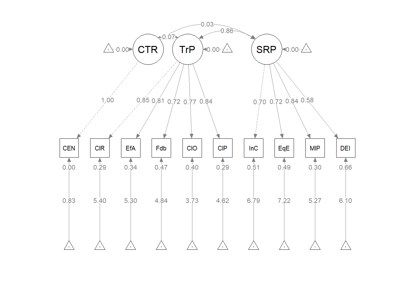
Results of the evaluation of the measurement model can be exported as .csv files with the following code. These produce output that inglude global fit indices, parameter estimates, and correlations between the latent variables, respetively. The tidySEM::table_fit function will display all of the global fit indices.
# global fit indices
init_msmt_fitstats <- tidySEM::table_fit(init_msmt_fit)
write.csv(init_msmt_fitstats, file = "init_msmt_fitstats.csv")
# parameter estimates
init_msmt_pEsts <- tidySEM::table_results(init_msmt_fit, digits = 3, columns = NULL)
write.csv(init_msmt_pEsts, file = "init_msmt_pEsts.csv")
# correlations between latent variables
init_msmt_LVcorr <- tidySEM::table_cors(init_msmt_fit, digits = 3)
write.csv(init_msmt_LVcorr, file = "init_msmt_LVcorr.csv")
Specify and evaluate a measurement model with either the subscale or randomly assigned to 3 parcels approaches
Each dataset has its unique challenges. This one has relatively few items per scale. I will therefore:
- Retain the single item indicator for CENTERING.
- Randomly assign the 5 items of the TradPed scale to 3 parcels (for parcels with 2, 2, and 1 member each)
- I don’t actually know that this is the best solution, but I will do it for demonstration purposes.
- Retain the four items as indicators for SRPed.
Here I assign the TradPed items to the 3 parcels.
set.seed(230916)
items <- c("ClearResponsibilities", "EffectiveAnswers", "Feedback", "ClearOrganization",
    "ClearPresentation")
parcels <- c("p1_TR", "p2_TR", "p3_TR")
data.frame(items = sample(items), parcel = rep(parcels, length = length(items)))
## items parcel
## 1 ClearPresentation p1_TR
## 2 Feedback p2_TR
## 3 ClearResponsibilities p3_TR
## 4 EffectiveAnswers p1_TR
## 5 ClearOrganization p2_TRI can now create the parcels using the traditional scoring procedure. I want both items to be present to score, so I will leave the .75 requirement (as a placeholder).
As a variable, ClearResponsibilities will stand alone (i.e., the scoring mechanism won’t work on a single variable).
TRp1_vars <- c("ClearPresentation", "EffectiveAnswers")
TRp2_vars <- c("Feedback", "ClearOrganization")

babydf$p1_TR <- sjstats::mean_n(babydf[, ..TRp1_vars], 0.75)
babydf$p2_TR <- sjstats::mean_n(babydf[, ..TRp2_vars], 0.75)

# If the scoring code above does not work for you, try the format
# below which involves removing the periods in front of the variable
# list. One example is provided. babydf$p3_TR <-
# sjstats::mean_n(babydf[, TRp3_vars], .75)
parc_msmt_mod <- "
##measurement model
CTR =~ CENTERING #this is a single item indicator, I had to add code below to set the variance
TradPed =~ p1_TR + p2_TR + ClearResponsibilities
SRPed =~ InclusvClassrm + EquitableEval + MultPerspectives + DEIintegration
# Variance of the single item indicator
CENTERING ~~ 0*CENTERING
# Covariances
CTR ~~ TradPed
CTR ~~ SRPed
TradPed ~~ SRPed
"
set.seed(230916)
parc_msmt_fit <- lavaan::cfa(parc_msmt_mod, data = babydf, missing = "fiml")
parc_msmt_fit_sum <- lavaan::summary(parc_msmt_fit, fit.measures = TRUE,
standardized = TRUE)
parc_msmt_fit_sum## lavaan 0.6.17 ended normally after 59 iterations
##
## Estimator ML
## Optimization method NLMINB
## Number of model parameters 26
##
## Number of observations 310
## Number of missing patterns 13
##
## Model Test User Model:
##
## Test statistic 112.981
## Degrees of freedom 18
## P-value (Chi-square) 0.000
##
## Model Test Baseline Model:
##
## Test statistic 1292.176
## Degrees of freedom 28
## P-value 0.000
##
## User Model versus Baseline Model:
##
## Comparative Fit Index (CFI) 0.925
## Tucker-Lewis Index (TLI) 0.883
##
## Robust Comparative Fit Index (CFI) 0.920
## Robust Tucker-Lewis Index (TLI) 0.875
##
## Loglikelihood and Information Criteria:
##
## Loglikelihood user model (H0) -2051.356
## Loglikelihood unrestricted model (H1) -1994.866
##
## Akaike (AIC) 4154.713
## Bayesian (BIC) 4251.863
## Sample-size adjusted Bayesian (SABIC) 4169.401
##
## Root Mean Square Error of Approximation:
##
## RMSEA 0.130
## 90 Percent confidence interval - lower 0.108
## 90 Percent confidence interval - upper 0.154
## P-value H_0: RMSEA <= 0.050 0.000
## P-value H_0: RMSEA >= 0.080 1.000
##
## Robust RMSEA 0.138
## 90 Percent confidence interval - lower 0.115
## 90 Percent confidence interval - upper 0.162
## P-value H_0: Robust RMSEA <= 0.050 0.000
## P-value H_0: Robust RMSEA >= 0.080 1.000
##
## Standardized Root Mean Square Residual:
##
## SRMR 0.062
##
## Parameter Estimates:
##
## Standard errors Standard
## Information Observed
## Observed information based on Hessian
##
## Latent Variables:
## Estimate Std.Err z-value P(>|z|) Std.lv Std.all
## CTR =~
## CENTERING 1.000 0.491 1.000
## TradPed =~
## p1_TR 1.000 0.702 0.870
## p2_TR 1.069 0.055 19.427 0.000 0.750 0.869
## ClearRspnsblts 1.000 0.052 19.076 0.000 0.702 0.855
## SRPed =~
## InclusvClassrm 1.000 0.475 0.699
## EquitableEval 0.959 0.088 10.922 0.000 0.455 0.719
## MultPerspectvs 1.474 0.117 12.561 0.000 0.700 0.839
## DEIintegration 0.905 0.100 9.089 0.000 0.430 0.582
##
## Covariances:
## Estimate Std.Err z-value P(>|z|) Std.lv Std.all
## CTR ~~
## TradPed -0.024 0.021 -1.152 0.249 -0.069 -0.069
## SRPed 0.008 0.015 0.523 0.601 0.033 0.033
## TradPed ~~
## SRPed 0.287 0.033 8.646 0.000 0.861 0.861
##
## Intercepts:
## Estimate Std.Err z-value P(>|z|) Std.lv Std.all
## .CENTERING 0.406 0.028 14.570 0.000 0.406 0.828
## .p1_TR 4.300 0.046 93.680 0.000 4.300 5.332
## .p2_TR 4.116 0.049 83.545 0.000 4.116 4.767
## .ClearRspnsblts 4.439 0.047 94.888 0.000 4.439 5.405
## .InclusvClassrm 4.613 0.039 118.347 0.000 4.613 6.786
## .EquitableEval 4.572 0.036 126.727 0.000 4.572 7.216
## .MultPerspectvs 4.391 0.048 92.290 0.000 4.391 5.265
## .DEIintegration 4.512 0.044 102.459 0.000 4.512 6.106
##
## Variances:
## Estimate Std.Err z-value P(>|z|) Std.lv Std.all
## .CENTERING 0.000 0.000 0.000
## .p1_TR 0.158 0.019 8.404 0.000 0.158 0.243
## .p2_TR 0.183 0.022 8.492 0.000 0.183 0.245
## .ClearRspnsblts 0.182 0.020 8.974 0.000 0.182 0.270
## .InclusvClassrm 0.237 0.023 10.252 0.000 0.237 0.512
## .EquitableEval 0.194 0.019 10.203 0.000 0.194 0.483
## .MultPerspectvs 0.205 0.026 7.845 0.000 0.205 0.295
## .DEIintegration 0.361 0.034 10.531 0.000 0.361 0.662
## CTR 0.241 0.019 12.450 0.000 1.000 1.000
## TradPed 0.493 0.053 9.361 0.000 1.000 1.000
## SRPed 0.226 0.035 6.513 0.000 1.000 1.000Interpret the results
| Criteria | Our Results | Criteria met? |
|---|---|---|
| Factor loadings significant, strong, proper valence | all \(p < 0.001\), lowest = .430(SRPed) | Yes |
| Non-significant chi-square | \(\chi ^{2}(18)= 112.982, p < 0.001\) | No |
| \(CFI\geq .95\) (or at least .90) | CFI = 0.925 | Almost! |
| \(RMSEA\leq .05\) (or < .08, at least < .10, also 90CI) | RMSEA = 0.130, 90CI[0.108, 0.154] | Worsened! |
| \(SRMR\leq .08\) (at least < .10) | SRMR = 0.062 | Worsened! |
| Combination rule: \(CFI \geq .95\) & \(SRMR \leq .08\) | CFI = 0.925, SRMR = 0.062 | No |
Results were mixed and somewhat worse than the initial model that included all item-level indicators. Here is the fit string: \(\chi^2(18)= 112.982, p < 0.001, CFI = 0.925, RMSEA = 0.130, 90CI[0.108, 0.154], SRMR = 0.062\)
semPlot::semPaths(parc_msmt_fit, what = "col", whatLabels = "stand", sizeMan = 5,
    node.width = 1, edge.label.cex = 0.75, style = "lisrel", mar = c(5,
        5, 5, 5))
# global fit indices
parc_msmt_fitstats <- tidySEM::table_fit(parc_msmt_fit)
write.csv(parc_msmt_fitstats, file = "parc_msmt_fitstats.csv")
# parameter estimates
parc_msmt_pEsts <- tidySEM::table_results(parc_msmt_fit, digits = 3, columns = NULL)
write.csv(parc_msmt_pEsts, file = "parc_msmt_pEsts.csv")
# correlations between latent variables
parc_msmt_LVcorr <- tidySEM::table_cors(parc_msmt_fit, digits = 3)
write.csv(parc_msmt_LVcorr, file = "parc_msmt_LVcorr.csv")
Make notes about similarities and differences in the all-items and parceled approaches
- Chi square was significant for both. A statistically significant chi-square is bad – it means that our measurement model covariance matrix is statistically significantly different than the sample covariance matrix.
- The CFI improved a tiny bit for the parcelled model.
- The RMSEA and SRMR worsened a tiny bit for the parcelled model.
Given that I didn’t really have enough items to parcel and the fit worsened for some of the indicators for the parcelled model, I think I will stay with the measurement model with item-level indicators. When I created the scales for the course evaluations, I was mindful of degrees of freedom and identification status of the model and intentionally chose to have a few items.
APA style results with table and figure
Analyzing our proposed multiple mediator model followed the two-step procedure of first evaluating a measurement model with acceptable fit to the data and then proceeding to test the structural model. Given that different researchers recommend somewhat differing thresholds to determine the adequacy of fit, We used the following as evidence of good fit: comparative fit indix (CFI) \(\geq 0.95\), root-mean-square error of approximation (RMSEA) \(\leq 0.06\), and the standard root-mean-square residual (SRMR) \(\leq 0.08\). To establish aceptable fit, we used CFI \(\geq 0.90\), RMSEA \(\leq 0.10\), and SRMR \(\leq 0.10\) (Weston & Gore, 2006).
We evaluated the measurement model by following recommendations by Little et al. (T. D. Little et al., 2002, 2013). Specificaly, each latent variable was represented by each of the items on its subscale. Given that TradPed and SRPed had 5 and 4 items, respectively, we did not parcel items. The Centering variable with two levels (pre-centered, re-centered) was recoded as a dummy variable with 0, 1 coding. In the specification, its measurement error was fixed at zero. While all factor loadings were strong, statistically significant, and properly valanced, global fit statistics were mixed: \(\chi^2(33)= 178.307, p < 0.001, CFI = 0.911, RMSEA = 0.119, 90CI[0.102, 0.137], SRMR = 0.060\). We proceeded to testing the strutural model with caution.
Table 1
| Factor Loadings for the Measurement Model |
|---|
| Latent variable and indicator | est | SE | p | est_std |
| Traditional Pedagogy | ||||
| ClearResponsibilities | 1.000 | 0.000 | 0.845 | |
| EffectiveAnswers | 0.967 | 0.056 | <0.001 | 0.815 |
| Feedback | 0.915 | 0.063 | <0.001 | 0.725 |
| ClearOrganization | 1.193 | 0.075 | <0.001 | 0.771 |
| ClearPresentation | 1.111 | 0.063 | <0.001 | 0.841 |
| Socially Responsive Pedagogy | ||||
| InclusvClassrm | 1.000 | 0.000 | 0.702 | |
| EquitableEval | 0.953 | 0.087 | <0.001 | 0.717 |
| MultPerspectives | 1.466 | 0.116 | <0.001 | 0.839 |
| DEIintegration | 0.901 | 0.099 | <0.001 | 0.582 |
| CENTERING | 0.000 | 0.000 | 0.000 |