Chapter 8 Moderated Mediation
The focus of this lecture is the moderated mediation. That is, are the effects of the indirect effect (sign, significance, strength, presence/absence) conditional on the effects of the moderator.
At the outset, please note that although I rely heavily on Hayes (2022a) text and materials, I am using the R package lavaan in these chapters. Recently, Hayes has introduced a PROCESS macro for R. Because I am not yet up-to-speed on using this macro (it is not a typical R package) and because we will use lavaan for confirmatory factor analysis and structural equation modeling, I have chosen to utilize the lavaan package. A substantial difference is that the PROCESS macros use ordinary least squares and lavaan uses maximum likelihood estimators.
8.2 Conditional Process Analysis
8.2.1 The definitional and conceptual
Hayes (Hayes, 2022a) coined the term and suggests we also talk about “conditional process modeling.”
Conditional process analysis: used when the analytical goal is to describe and understand the conditional nature of the mechanism or mechanisms by which a variable transmits its effect on another.
We are integrating moderation and mediation mechanisms together into a single integrated analytical model.
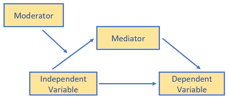
- Mediator: Any causal system in which at least one causal antecedent X variable is proposed as influencing an outcome Y through a intervening variable M. In this model, there are two pathways by which X can influence Y: direct effect of X on Y, and indirect effect of X on Y through M.
- Answers question, “How does X affect Y”
- Partitions the X-to-Y relationship into two paths of influence: direct, indirect.
- Indirect effect contains two components (a,b) that when multipled (a*b) yield an estimate of how much these two cases that differ by one unit on X are estimated to differ on Y through the effect of X on M, which in turn affects Y.
- Keywords: how, through, via, indirect effect
- Moderator: The effect of X on some variable Y is moderated by W if its size, sign, or strength depends on or can be predicted by W.
- Stated another way, W and X interact in their influence on Y.
- Moderators help establish the boundary conditions of an effect or the circumstances, stimuli, or type of people for which the effect is large v. small, present v. absent, positive v. negative, and so forth.
- Keywords: “it depends,” interaction effect.
- Stated another way, W and X interact in their influence on Y.
Why should we engage both mediators and moderators? Hayes (2022a) suggest that if we have only a mediator(s) in the model that we lose information if we “reduce complex responses that no doubt differ from person to person or situation to situation” (p. 394). He adds that “all effects are moderated by something” (p. 394). Correspondingly, he recommends we add them to a mediation anlaysis.
Hayes (2022a) suggests that “more complete” (p. 395) analyses model the mechanisms at work linking X to Y (mediator[s]) while simultaneously allowing those effects to be contingent on context, circumstance, or individual difference (moderator[s]).
What are conditional direct and indirect effects?. Mediation analyses produce indirect (the product of a sequence of effects that are assumed to be causal) and direct (the unique contribution of X to Y, controlling for other variables in the model) effects. These effects (the X-to-Y/direct and X-to-M-to-Y/indirect), can also be moderated. This is our quest! Figure 11.2 in Hayes’ text (2022a) illustrates conceptually and statistically that we can specify moderation of any combination of direct and indirect paths/effects.
Within the CPA framework we have lots of options that generally fall into two categories:
- Moderated mediation: when an indirect effect of X on Y through M is moderated; the mechanism represented by the X-to-M-to-Y chain of events operates to varying degrees (or not at all) for certain people or in certain contexts.
- Any model in which the indirect effect (a*b) changes as a function of one or more moderators. These moderators can be operating on the a, b, or c’ paths or any possible combination of the three
- X could moderate its own indirect effect on Y through M if the effect of M on Y depends on X, or
- The indirect effect of X on Y through M could be contingent on a fourth variable if that fourth variable W moderates one or more of the relationships in a three-variable causal system, or
- An indirect effect could be contingent on a moderator variable
- Mediated moderation: an interaction between X and some moderator W on Y is carried through a mediator M;
- mediated moderation analysis is simply a mediation analysis with the product of two variables serving as the causal agent of focus
- An interaction between a moderator W and causal agent X on outcome Y could operate through a mediator M
Hayes argues that the mediated moderation hypotheses are “regularly articulated and tested by scientists” (2022a, p. 459). He warns, though, that we should not confuse the “abundance of published examples of mediated moderation analyses…with the meaningfulness of the procedure itself” (p. 460). He later adds that mediation moderation is “neither interesting nor meaningful.” Why?
- Conceptualizing a process in terms of a mediated moderation misdirects attention toward a variable in the model that actually doesn’t measure anything.
- Most often there are moderated mediation models that are identical in equations and resulting coefficients - the difference is in the resulting attentional focus and interpretation.
- Hayes (2022a) recommends that models proposing mediated moderation be recast in terms of moderated mediation process.
- Consequently, we will not work a mediated moderation, but there is an example in his text.
8.3 Workflow for Moderated Mediation
 Conducting a moderated mediation involves the following steps:
- Conducting an a priori power analysis to determine the appropriate sample size.
- This will require estimates of effect that are drawn from pilot data, the literature, or both.
- Scrubbing and scoring the data.
- Guidelines for such are presented in the respective lessons.
- Conducting data diagnostics, this includes:
- item and scale level missingness,
- internal consistency coefficients (e.g., alphas or omegas) for scale scores,
- univariate and multivariate normality
- Beginning with a piecewise analysis of the simpler mediation and moderation(s) models in the larger model.
- Make note of findings in each of the smaller models.
- Changes in significance of results from smaller to larger models may indicate power problems and/or combinatorial effects of the variables.
- Specifying and run the model overall model (this lesson presumes it will with the R package, lavaan).
- The dependent variable should be predicted by the independent, mediating, and covarying (if any) variables and any of their proposed interactions.
- “Labels” can facilitate interpretation by naming the a, b, and c’ paths.
- Script should include calculations for the index of moderated mediation and conditional indirect and direct (if included in the model) effects.
- Conducting a post hoc power analysis.
- Informed by your own results, you can see if you were adequately powered to detect a statistically significant effect, if, in fact, one exists.
- Interpret and report the results.
- Interpret ALL the paths and their patterns.
- Report if some indirect effects are stronger than others (i.e., results of the contrasts).
- Create a table and figure.
- Prepare the results in a manner that is useful to your audience.
In this workflow I call your attention to Hayes’ (2022a) piecewise approach to building models. I embrace this approach for a number of reasons. One reason is that examining the smaller portions of the model allows us to really begin to understand the patterns in the data in a systematic way.
Another reason I appreciate the piecewise approach are our historically rigid traditions around hypothesis testing. In summarizing a strategic approach for testing structural equation models, Joreskog (Joreskog, 1993) identified three scenarios:
- strictly confirmatory: the traditional NHST approach of proposing a single, theoretically derived, model, and after analyzing the data either rejects or fails to reject the model. No further modifications are made/allowed.
- alternative models: the reseacher proposes competing (also theoretically derived) models. Following analysis of a single set of empirical data, he or she selects one model as appropriate in representing the sample data.
- model generating: A priori, the researcher acknowledges that they may/may not find what they have theoretically proposed. So, a priori, they acknowledge that in the absence of ideal fit (which is the usual circumstance), they will proceed in an exploratory fashion to respecify/re-estimate the model. The goal is to find a model that is both substantively meaningful and statistically well-fitting.
A legacy of our field is the strictly confirmatory approach. I am thrilled when I see research experts (e.g., (Byrne, 2016c)) openly endorse a model building approach.
8.4 Research Vignette
Once again the research vignette comes from the Lewis, Williams, Peppers, and Gadson’s (2017) study titled, “Applying Intersectionality to Explore the Relations Between Gendered Racism and Health Among Black Women.” The study was published in the Journal of Counseling Psychology. Participants were 231 Black women who completed an online survey.
Variables used in the study included:
GRMS: Gendered Racial Microaggressions Scale (J. A. Lewis & Neville, 2015) is a 26-item scale that assesses the frequency of nonverbal, verbal, and behavioral negative racial and gender slights experienced by Black women. Scaling is along six points ranging from 0 (never) to 5 (once a week or more). Higher scores indicate a greater frequency of gendered racial microaggressions. An example item is, “Someone has made a sexually inappropriate comment about my butt, hips, or thighs.”
MntlHlth and PhysHlth: Short Form Health Survey - Version 2 (Ware et al., 1995) is a 12-item scale used to report self-reported mental (six items) and physical health (six items). Higher scores indicate higher mental health (e.g., little or no psychological ldistress) and physical health (e.g., little or no reported symptoms in physical functioning). An example of an item assessing mental health was, “How much of the time during the last 4 weeks have you felt calm and peaceful?”; an example of a physical health item was, “During the past 4 weeks, how much did pain interfere with your normal work?”
Sprtlty, SocSup, Engmgt, and DisEngmt are four subscales from the Brief Coping with Problems Experienced Inventory (Carver, 1997). The 28 items on this scale are presented on a 4-point scale ranging from 1 (I usually do not do this at all) to 4(I usually do this a lot). Higher scores indicate a respondents’ tendency to engage in a particular strategy. Instructions were modified to ask how the female participants responded to recent experiences of racism and sexism as Black women. The four subscales included spirituality (religion, acceptance, planning), interconnectedness/social support (vent emotions, emotional support,instrumental social support), problem-oriented/engagement coping (active coping, humor, positive reinterpretation/positive reframing), and disengagement coping (behavioral disengagement, substance abuse, denial, self-blame, self-distraction).
GRIcntlty: The Multidimensional Inventory of Black Identity Centrality subscale (Sellers et al., n.d.) was modified to measure the intersection of racial and gender identity centrality. The scale included 10 items scaled from 1 (strongly disagree) to 7 (strongly agree). An example item was, “Being a Black woman is important to my self-image.” Higher scores indicated higher levels of gendered racial identity centrality.
8.4.1 Simulating the data from the journal article
The lavaan::simulateData function was used. If you have taken psychometrics, you may recognize the code as one that creates latent variables form item-level data. In trying to be as authentic as possible, we retrieved factor loadings from psychometrically oriented articles that evaluated the measures (Nadal, 2011; Veit & Ware, 1983). For all others we specified a factor loading of 0.80. We then approximated the measurement model by specifying the correlations between the latent variable. We sourced these from the correlation matrix from the research vignette (J. A. Lewis et al., 2017). The process created data with multiple decimals and values that exceeded the boundaries of the variables. For example, in all scales there were negative values. Therefore, the final element of the simulation was a linear transformation that rescaled the variables back to the range described in the journal article and rounding the values to integer (i.e., with no decimal places).
#Entering the intercorrelations, means, and standard deviations from the journal article


Lewis_generating_model <- '
        #measurement model
        GRMS  =~ .69*Ob1 + .69*Ob2 + .60*Ob3 + .59*Ob4 + .55*Ob5 + .55*Ob6 + .54*Ob7 + .50*Ob8 + .41*Ob9 + .41*Ob10 + .93*Ma1 + .81*Ma2 + .69*Ma3 + .67*Ma4 + .61*Ma5 + .58*Ma6 + .54*Ma7 + .59*St1 + .55*St2 + .54*St3 + .54*St4 + .51*St5 + .70*An1 + .69*An2 + .68*An3
        MntlHlth  =~ .8*MH1 + .8*MH2 + .8*MH3 + .8*MH4 + .8*MH5 + .8*MH6
        PhysHlth  =~ .8*PhH1 + .8*PhH2 + .8*PhH3 + .8*PhH4 + .8*PhH5 + .8*PhH6
        Spirituality  =~ .8*Spirit1 + .8*Spirit2
        SocSupport  =~ .8*SocS1 + .8*SocS2
        Engagement  =~ .8*Eng1 + .8*Eng2
        Disengagement  =~  .8*dEng1 + .8*dEng2
        GRIC  =~ .8*Cntrlty1 + .8*Cntrlty2 + .8*Cntrlty3 + .8*Cntrlty4 + .8*Cntrlty5 + .8*Cntrlty6 + .8*Cntrlty7 + .8*Cntrlty8 + .8*Cntrlty9 + .8*Cntrlty10

        #Means
         GRMS ~ 1.99*1
         Spirituality ~2.82*1
         SocSupport ~ 2.48*1
         Engagement ~ 2.32*1
         Disengagement ~ 1.75*1
         GRIC ~ 5.71*1
         MntlHlth ~3.56*1 #Lewis et al used sums instead of means, I recast as means to facilitate simulation
         PhysHlth ~ 3.51*1 #Lewis et al used sums instead of means, I recast as means to facilitate simulation

        #Correlations
         GRMS ~ 0.20*Spirituality
         GRMS ~ 0.28*SocSupport
         GRMS ~ 0.30*Engagement
         GRMS ~ 0.41*Disengagement
         GRMS ~ 0.19*GRIC
         GRMS ~ -0.32*MntlHlth
         GRMS ~ -0.18*PhysHlth

         Spirituality ~ 0.49*SocSupport
         Spirituality ~ 0.57*Engagement
         Spirituality ~ 0.22*Disengagement
         Spirituality ~ 0.12*GRIC
         Spirituality ~ -0.06*MntlHlth
         Spirituality ~ -0.13*PhysHlth

         SocSupport ~ 0.46*Engagement
         SocSupport ~ 0.26*Disengagement
         SocSupport ~ 0.38*GRIC
         SocSupport ~ -0.18*MntlHlth
         SocSupport ~ -0.08*PhysHlth

         Engagement ~ 0.37*Disengagement
         Engagement ~ 0.08*GRIC
         Engagement ~ -0.14*MntlHlth
         Engagement ~ -0.06*PhysHlth

         Disengagement ~ 0.05*GRIC
         Disengagement ~ -0.54*MntlHlth
         Disengagement ~ -0.28*PhysHlth

         GRIC ~ -0.10*MntlHlth
         GRIC ~ 0.14*PhysHlth

         MntlHlth ~ 0.47*PhysHlth
        '

set.seed(230925)
dfLewis <- lavaan::simulateData(model = Lewis_generating_model,
                              model.type = "sem",
                              meanstructure = T,
                              sample.nobs=231,
                              standardized=FALSE)

#used to retrieve column indices used in the rescaling script below
#col_index <- as.data.frame(colnames(dfLewis))

for(i in 1:ncol(dfLewis)){  # for loop to go through each column of the dataframe
  if(i >= 1 & i <= 25){   # apply only to GRMS variables
    dfLewis[,i] <- scales::rescale(dfLewis[,i], c(0, 5))
  }
  if(i >= 26 & i <= 37){   # apply only to mental and physical health variables
    dfLewis[,i] <- scales::rescale(dfLewis[,i], c(0, 6))
  }
  if(i >= 38 & i <= 45){   # apply only to coping variables
    dfLewis[,i] <- scales::rescale(dfLewis[,i], c(1, 4))
  }
  if(i >= 46 & i <= 55){   # apply only to GRIC variables
    dfLewis[,i] <- scales::rescale(dfLewis[,i], c(1, 7))
  }
}

#rounding to integers so that the data resembles that which was collected
library(tidyverse)
dfLewis <- dfLewis %>% round(0)

#quick check of my work
#psych::describe(dfLewis)
The script below allows you to store the simulated data as a file on your computer. This is optional – the entire lesson can be worked with the simulated data.
If you prefer the .rds format, use this script (remove the hashtags). The .rds format has the advantage of preserving any formatting of variables. A disadvantage is that you cannot open these files outside of the R environment.
Script to save the data to your computer as an .rds file.
Once saved, you could clean your environment and bring the data back in from its .csv format.
If you prefer the .csv format (think “Excel lite”) use this script (remove the hashtags). An advantage of the .csv format is that you can open the data outside of the R environment. A disadvantage is that it may not retain any formatting of variables
Script to save the data to your computer as a .csv file.
Once saved, you could clean your environment and bring the data back in from its .csv format.
8.4.2 Scrubbing, Scoring, and Data Diagnostics
Because the focus of this lesson is on moderation, we have used simulated data (which serves to avoid problems like missingness and non-normal distributions). If this were real, raw, data, it would be important to scrub, score, and conduct data diagnostics to evaluate the suitability of the data for the proposes anlayses.
Because we are working with item level data we do need to score the scales used in the researcher’s model. Because we are using simulated data and the authors already reverse coded any such items, we will omit that step.
As described in the Scoring chapter, we calculate mean scores of these variables by first creating concatenated lists of variable names. Next we apply the sjstats::mean_n function to obtain mean scores when a given percentage (we’ll specify 80%) of variables are non-missing. Functionally, this would require the two-item variables (e.g., engagement coping and disengagement coping) to have non-missingness. We simulated a set of data that does not have missingness, none-the-less, this specification is useful in real-world settings.
Note that I am only scoring the variables used in the models demonstrated in this lesson. The variables that are simulated but not scored could be used for the practice suggestions.
GRMS_vars <- c("Ob1", "Ob2", "Ob3", "Ob4", "Ob5", "Ob6", "Ob7", "Ob8",
    "Ob9", "Ob10", "Ma1", "Ma2", "Ma3", "Ma4", "Ma5", "Ma6", "Ma7", "St1",
    "St2", "St3", "St4", "St5", "An1", "An2", "An3")
Eng_vars <- c("Eng1", "Eng2")
dEng_vars <- c("dEng1", "dEng2")
MntlHlth_vars <- c("MH1", "MH2", "MH3", "MH4", "MH5", "MH6")
Cntrlty_vars <- c("Cntrlty1", "Cntrlty2", "Cntrlty3", "Cntrlty4", "Cntrlty5",
    "Cntrlty6", "Cntrlty7", "Cntrlty8", "Cntrlty9", "Cntrlty10")

dfLewis$GRMS <- sjstats::mean_n(dfLewis[, GRMS_vars], 0.8)
## Registered S3 methods overwritten by 'broom':
## method from
## tidy.glht jtools
## tidy.summary.glht jtoolsdfLewis$Engmt <- sjstats::mean_n(dfLewis[, Eng_vars], 0.8)
dfLewis$DisEngmt <- sjstats::mean_n(dfLewis[, dEng_vars], 0.8)
dfLewis$MntlHlth <- sjstats::mean_n(dfLewis[, MntlHlth_vars], 0.8)
dfLewis$Centrality <- sjstats::mean_n(dfLewis[, Cntrlty_vars], 0.8)
# If the scoring code above does not work for you, try the format
# below which involves inserting to periods in front of the variable
# list. One example is provided. dfLewis$GRMS <-
# sjstats::mean_n(dfLewis[, ..GRMS_vars], 0.80)Now that we have scored our data, let’s trim the variables to just those we need.
Let’s check a table of means, standard deviations, and correlations to see if they align with the published article.
Lewis_table <- apaTables::apa.cor.table(Lewis_df, table.number = 1, show.sig.stars = TRUE,
    landscape = TRUE, filename = "Lewis_Corr.doc")
print(Lewis_table)
##
##
## Table 1
##
## Means, standard deviations, and correlations with confidence intervals
##
##
## Variable M SD 1 2 3
## 1. GRMS 2.56 0.72
##
## 2. Centrality 3.94 0.76 .24**
## [.11, .36]
##
## 3. DisEngmt 2.48 0.52 .53** .05
## [.43, .62] [-.08, .18]
##
## 4. MntlHlth 3.16 0.81 -.56** -.09 -.48**
## [-.64, -.47] [-.21, .04] [-.57, -.37]
##
##
## Note. M and SD are used to represent mean and standard deviation, respectively.
## Values in square brackets indicate the 95% confidence interval.
## The confidence interval is a plausible range of population correlations
## that could have caused the sample correlation (Cumming, 2014).
## * indicates p < .05. ** indicates p < .01.
## 8.4.3 Quick peek at the data
##            vars   n mean   sd median trimmed  mad  min  max range  skew
## GRMS          1 231 2.56 0.72   2.56    2.56 0.77 0.32 4.24  3.92 -0.08
## Centrality    2 231 3.94 0.76   3.90    3.92 0.74 1.90 6.00  4.10  0.25
## DisEngmt      3 231 2.48 0.52   2.50    2.47 0.74 1.00 4.00  3.00  0.11
## MntlHlth      4 231 3.16 0.81   3.17    3.16 0.74 1.17 5.50  4.33  0.05
##            kurtosis   se
## GRMS          -0.14 0.05
## Centrality    -0.08 0.05
## DisEngmt      -0.16 0.03
## MntlHlth      -0.20 0.05
8.5 Working the Moderated Mediation
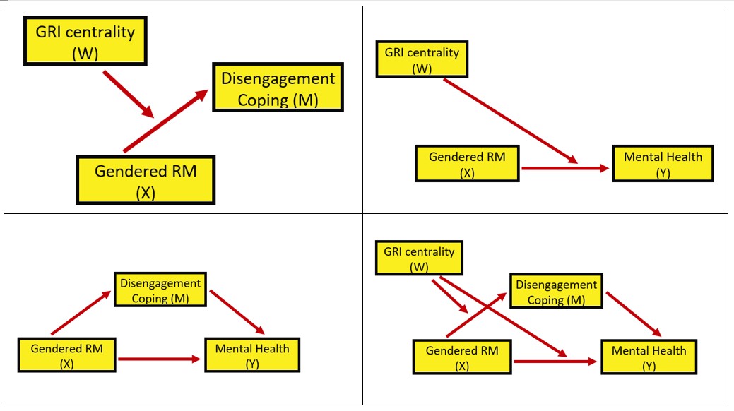
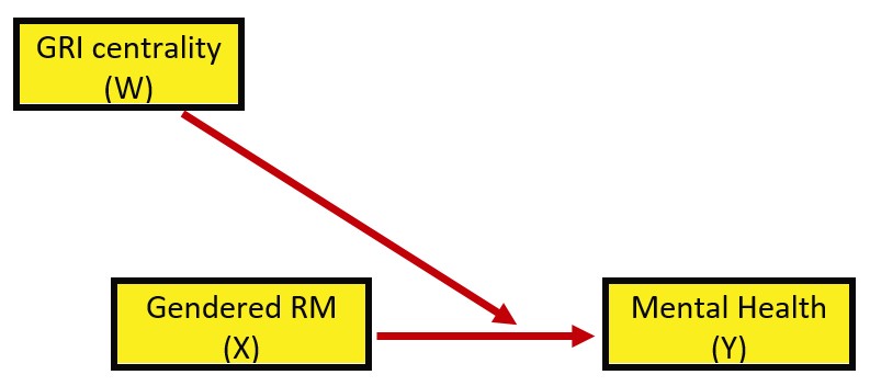
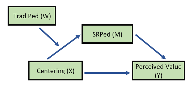
The model we are testing is predicting a mental health (MntlHlth, Y) from gendered racial microaggressions (GRMS,X), mediated by disengagement coping (DisEngmt, M). The relationship between gendered racial microaggressions and disengagement coping (i.e., the a path) is expected to be moderated by gendered racial identity centrality (GRIcntlty, W). Gendered racial identity centrality is also expected to moderate the path between gendered racial microaggressions and mental health (i.e., the c’ path). Thus, the specified model involves the evaluation of a conditional indirect effect.
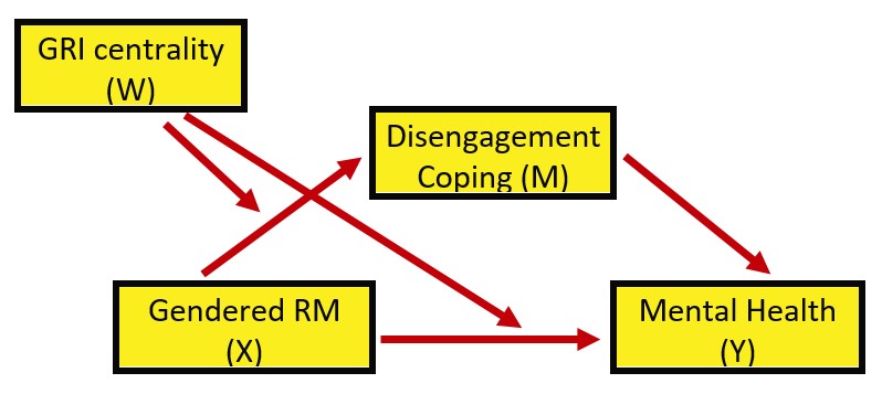
Hayes’ (2022a) textbook and training materials frequently display the conceptual (above) and statistical models (below). These help facilitate understanding.
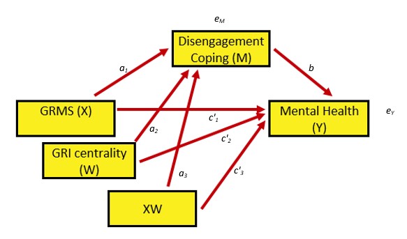
Looking at the diagram, with two consequent variables (i.e., those with arrows pointing to them) we can see two equations are needed to explain the model:
\[M = i_{M}+a_{1}X + a_{2}W + a_{3}XW + e_{M}\]
\[Y = i_{Y}+c_{1}^{'}X+ c_{2}^{'}W+c_{3}^{'}XW+ bM+e_{Y}\]
When we have complicated models such as these, Hayes (2022a) suggests a piecewise approach to model building. Specifically, he decompose the model into its aggregate parts: a simple mediation and two simple moderation.
Let’s start with the the simple moderations.
8.5.1 Piecewise Assembly of the Moderated Mediation
8.5.1.1 Analysis #1: A simple moderation
We are asking, “Does GRI centrality moderate the relationship between gendered racial microaggressions and disengagement coping?
Y = disengagement coping X = gendered racial microaggressions W = GRI centrality
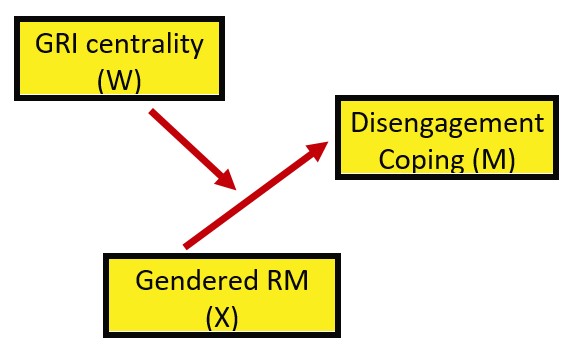
The formula we are estimating: \[Y=b_{0}+b_{1}X+b_{2}W+b_{3}XW+e_{Y}\]
Let’s specify this simple moderation model with base R’s lm() function. Let’s use the jtools package so we get that great summ function and interactions for the awesome plot.
Since we are just working to understand our moderations, we can run them with “regular old” ordinary least squares.
# library(jtools) #the summ function creates a terrific regression
# table library(interactions) library(ggplot2)

Mod_a_path <- lm(DisEngmt ~ GRMS * Centrality, data = Lewis_df)
jtools::summ(Mod_a_path, digits = 3)| Observations | 231 |
| Dependent variable | DisEngmt |
| Type | OLS linear regression |
| F(3,227) | 31.245 |
| R² | 0.292 |
| Adj. R² | 0.283 |
| Est. | S.E. | t val. | p | |
|---|---|---|---|---|
| (Intercept) | 1.107 | 0.510 | 2.169 | 0.031 |
| GRMS | 0.623 | 0.193 | 3.220 | 0.001 |
| Centrality | 0.093 | 0.132 | 0.703 | 0.483 |
| GRMS:Centrality | -0.058 | 0.049 | -1.179 | 0.240 |
| Standard errors: OLS |
Looking at these results we can see that the predictors account for about 29% of variance in disengagement coping. Only the independent variable (X), GRMS is a significant predictor. Neither the moderator (GRIcntlty, [Y])), nor its interaction with GRMS (GRMS:GRIcntlty, [XW]) are significant.
It’s always helpful to graph the relationship. The interaction_plot() function from the package, interactions can make helpful illustrations. In the case of interactions/moderations, I like to run them “both ways” to see which makes more sense.
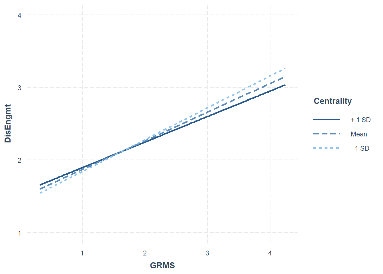 The figure with GRIcntrlty as the moderator, shows a very similar prediction of disengagement coping from gendered racial microaggressions across all three levels of gendered racial identity centrality.
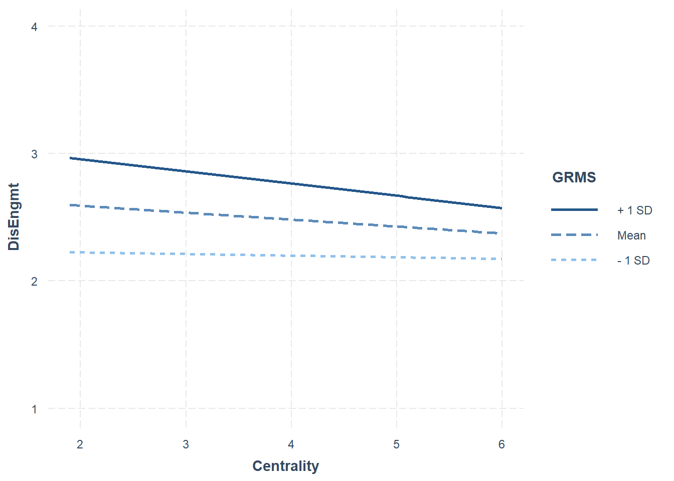
The figure that positions GRMS in the moderator role shows the significant main effect of GRMS on disengagement coping. It is clear that who experience the highest levels of gendered racial microaggressions are using a more disengaged coping style.
Next, let’s probe the interaction with simple slopes. Probing the interaction is a common follow-up. With these additional inferential tests we can see where in the distribution of the moderator, X has an effect on Y that is different from zero (and where it does not). There are two common approaches.
The Johnson-Neyman is a floodlight approach and provides an indication of the places in the distribution of W (moderator) that X has an effect on Y that is different than zero. The analysis of simple slopes approach is thought of as a spotlight approach because probes the distribution at specific values (often the M +/- 1SD).
## JOHNSON-NEYMAN INTERVAL
##
## When Centrality is INSIDE the interval [-6.39, 6.37], the slope of GRMS is
## p < .05.
##
## Note: The range of observed values of Centrality is [1.90, 6.00]
##
## SIMPLE SLOPES ANALYSIS
##
## Slope of GRMS when Centrality = 3.182522 (- 1 SD):
##
##   Est.   S.E.   t val.      p
## ------ ------ -------- ------
##   0.44   0.05     8.23   0.00
##
## Slope of GRMS when Centrality = 3.938095 (Mean):
##
##   Est.   S.E.   t val.      p
## ------ ------ -------- ------
##   0.40   0.04     9.42   0.00
##
## Slope of GRMS when Centrality = 4.693668 (+ 1 SD):
##
##   Est.   S.E.   t val.      p
## ------ ------ -------- ------
##   0.35   0.06     6.03   0.00
# sim_slopes(Mod_a_path, pred=GRIcntlty, modx = GRMS) #sometimes I
# like to look at it in reverse -- like in the plotsThe Johnson-Neyman suggests that between the GRIcntlty values of -6.39 and 6.37, the relationship between GRMS is statistically significant. We see the same result in the pick-a-point approach where at the GRIcntlty values of 3.18, 3.94, and 4.69, GRMS has a statistically significant effect on disengagement coping. Is this a contradiction to the non-significant interaction effect?
No. The test of interaction is an interaction about the relationship between W and X’s effect on Y. Just showing that X is significantly related to Y for a specific value does not address any dependence upon the moderator (W). Hayes (2022a) covers this well in his Chapter 14, in the section “Reporting a Moderation Analysis.”
What have we learned in this simple moderation?
- Only GRMS (X) has a statistically significant effect on disengagement coping.
- Neither the moderator (Centrality W) nor its interaction with GRMS (WX) are statistically significant. While there are no significant predictors (neither X, W, nor XW)
- The model accounts for about 29% of variance in the DV.
8.5.1.2 Analysis #2: Another simple moderation
We are asking, “Does gendered racial identity centrality moderate the relationship between gendered racial microaggressions and mental health?”
Y = mental health X = gendered racial microaggressions W = GRI centrality
As before, this is our formulaic rendering:
\[Y=b_{0}+b_{1}X+b_{2}W+b_{3}XW+e_{Y}\]
Mod_c_path <- lm(MntlHlth ~ GRMS * Centrality, data = Lewis_df)
jtools::summ(Mod_c_path, digits = 3)| Observations | 231 |
| Dependent variable | MntlHlth |
| Type | OLS linear regression |
| F(3,227) | 37.386 |
| R² | 0.331 |
| Adj. R² | 0.322 |
| Est. | S.E. | t val. | p | |
|---|---|---|---|---|
| (Intercept) | 6.138 | 0.767 | 8.007 | 0.000 |
| GRMS | -1.248 | 0.290 | -4.299 | 0.000 |
| Centrality | -0.351 | 0.199 | -1.764 | 0.079 |
| GRMS:Centrality | 0.157 | 0.073 | 2.132 | 0.034 |
| Standard errors: OLS |
In this model that is, overall, statistically significant, we account for about 33% of variance in the DV. Looking at these results we can see that there is a statistically significant main effect of GRMS on mental health as well as statistically significant GRMS:Centrality interaction effect.
Let’s look at the plots.
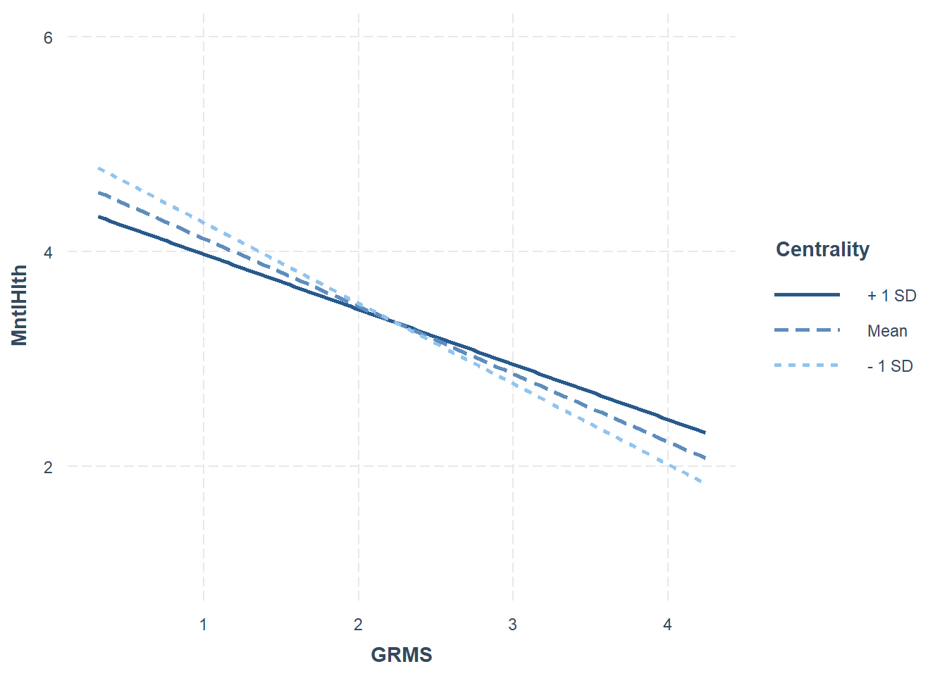
The figure with GRIcntrlty as the moderator, shows fanning out when mental health is high and GRMS is low.
Next, let’s probe the interaction with simple slopes. Probing the interaction is a common follow-up. With these additional inferential tests we can see where in the distribution of the moderator, X has an effect on Y that is different from zero (and where it does not). There are two common approaches.
The Johnson-Neyman is a floodlight approach and provides an indication of the places in the distribution of W (moderator) that X has an effect on Y that is different than zero. The analysis of simple slopes or spotlight approach, probes the distribution at specific values (often the M +/- 1SD).
## JOHNSON-NEYMAN INTERVAL
##
## When Centrality is OUTSIDE the interval [5.92, 58.37], the slope of GRMS is
## p < .05.
##
## Note: The range of observed values of Centrality is [1.90, 6.00]
##
## SIMPLE SLOPES ANALYSIS
##
## Slope of GRMS when Centrality = 3.182522 (- 1 SD):
##
##    Est.   S.E.   t val.      p
## ------- ------ -------- ------
##   -0.75   0.08    -9.36   0.00
##
## Slope of GRMS when Centrality = 3.938095 (Mean):
##
##    Est.   S.E.   t val.      p
## ------- ------ -------- ------
##   -0.63   0.06   -10.01   0.00
##
## Slope of GRMS when Centrality = 4.693668 (+ 1 SD):
##
##    Est.   S.E.   t val.      p
## ------- ------ -------- ------
##   -0.51   0.09    -5.85   0.00
# sim_slopes(Mod_c_path, pred=GRIcntlty, modx = GRMS) #sometimes I
# like to look at it in reverse -- like in the plotsThe Johnson-Neyman suggests that between the Centrality values of 5.92 and 58.37], the relationship between GRMS is and mental health statistically significant. We see the same result in the pick-a-point approach where at the Centrality values of 3.19, 3.94, and 4.69, GRMS has a statistically significant effect on mental health. Is this a contradiction to the non-significant interaction effect?
What have we learned in this simple moderation?
- There was a statistically significant main effect of GRMS on mental health as well as statistically significant GRMS:Centrality interaction effect.
- It is curious that in the presence of the statistically significant interaction effect, we did not see differences in significance in the analysis of simple slopes.
- The overall model was significant and accounted for 33% of variance in the DV.
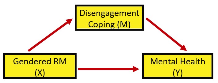
8.5.1.3 Analysis #3: A simple mediation
We are asking, “Does disengagement coping mediate the relationship between gendered racial microaggressions and mental health?”
Y = mental health X = gendered racial microaggressions M = GRI centrality
 Looking at the diagram, with two consequent variables (i.e., those with arrows pointing to them) we can see two equations are needed to explain the model:
\[M = i_{M}+aX + e_{M}\]
\[Y = i_{Y}+c'X+ bM+e_{Y}\]
To conduct this analysis, I am using the guidelines in the chapter on simple mediation. We are switching to the lavaan package.
library(lavaan)

LMedModel <- "
          MntlHlth ~ b*DisEngmt + c_p*GRMS
          DisEngmt ~a*GRMS

          #intercepts
          DisEngmt ~ DisEngmt.mean*1
          MntlHlth ~ MntlHlth.mean*1

          indirect :=  a*b
          direct  := c_p
          total_c  := c_p + (a*b)
          "
set.seed(230925)  #required for reproducible results because lavaan introduces randomness into the calculations
LMed_fit <- lavaan::sem(LMedModel, data = Lewis_df, se = "bootstrap", missing = "fiml")
LMed_Sum <- lavaan::summary(LMed_fit, standardized = T, rsq = T, ci = TRUE)
LMed_ParEsts <- lavaan::parameterEstimates(LMed_fit, boot.ci.type = "bca.simple",
    standardized = TRUE)
LMed_Sum
## lavaan 0.6.17 ended normally after 1 iteration
##
## Estimator ML
## Optimization method NLMINB
## Number of model parameters 7
##
## Number of observations 231
## Number of missing patterns 1
##
## Model Test User Model:
##
## Test statistic 0.000
## Degrees of freedom 0
##
## Parameter Estimates:
##
## Standard errors Bootstrap
## Number of requested bootstrap draws 1000
## Number of successful bootstrap draws 1000
##
## Regressions:
## Estimate Std.Err z-value P(>|z|) ci.lower ci.upper
## MntlHlth ~
## DisEngmt (b) -0.381 0.089 -4.262 0.000 -0.547 -0.206
## GRMS (c_p) -0.483 0.066 -7.271 0.000 -0.607 -0.354
## DisEngmt ~
## GRMS (a) 0.386 0.038 10.096 0.000 0.301 0.456
## Std.lv Std.all
##
## -0.381 -0.247
## -0.483 -0.430
##
## 0.386 0.531
##
## Intercepts:
## Estimate Std.Err z-value P(>|z|) ci.lower ci.upper
## .DsEngmt (DsE.) 1.490 0.100 14.935 0.000 1.307 1.709
## .MntlHlt (MnH.) 5.342 0.195 27.390 0.000 4.953 5.721
## Std.lv Std.all
## 1.490 2.845
## 5.342 6.604
##
## Variances:
## Estimate Std.Err z-value P(>|z|) ci.lower ci.upper
## .MntlHlth 0.420 0.040 10.544 0.000 0.343 0.496
## .DisEngmt 0.197 0.016 11.967 0.000 0.163 0.229
## Std.lv Std.all
## 0.420 0.641
## 0.197 0.718
##
## R-Square:
## Estimate
## MntlHlth 0.359
## DisEngmt 0.282
##
## Defined Parameters:
## Estimate Std.Err z-value P(>|z|) ci.lower ci.upper
## indirect -0.147 0.039 -3.824 0.000 -0.226 -0.075
## direct -0.483 0.067 -7.268 0.000 -0.607 -0.354
## total_c -0.631 0.058 -10.789 0.000 -0.742 -0.513
## Std.lv Std.all
## -0.147 -0.131
## -0.483 -0.430
## -0.631 -0.561## lhs op rhs label est se z pvalue ci.lower
## 1 MntlHlth ~ DisEngmt b -0.381 0.089 -4.262 0 -0.547
## 2 MntlHlth ~ GRMS c_p -0.483 0.066 -7.271 0 -0.606
## 3 DisEngmt ~ GRMS a 0.386 0.038 10.096 0 0.311
## 4 DisEngmt ~1 DisEngmt.mean 1.490 0.100 14.935 0 1.297
## 5 MntlHlth ~1 MntlHlth.mean 5.342 0.195 27.390 0 4.900
## 6 MntlHlth ~~ MntlHlth 0.420 0.040 10.544 0 0.352
## 7 DisEngmt ~~ DisEngmt 0.197 0.016 11.967 0 0.166
## 8 GRMS ~~ GRMS 0.518 0.000 NA NA 0.518
## 9 GRMS ~1 2.557 0.000 NA NA 2.557
## 10 indirect := a*b indirect -0.147 0.039 -3.824 0 -0.234
## 11 direct := c_p direct -0.483 0.067 -7.268 0 -0.606
## 12 total_c := c_p+(a*b) total_c -0.631 0.058 -10.789 0 -0.739
## ci.upper std.lv std.all std.nox
## 1 -0.206 -0.381 -0.247 -0.247
## 2 -0.347 -0.483 -0.430 -0.597
## 3 0.465 0.386 0.531 0.738
## 4 1.698 1.490 2.845 2.845
## 5 5.699 5.342 6.604 6.604
## 6 0.513 0.420 0.641 0.641
## 7 0.234 0.197 0.718 0.718
## 8 0.518 0.518 1.000 0.518
## 9 2.557 2.557 3.552 2.557
## 10 -0.079 -0.147 -0.131 -0.182
## 11 -0.347 -0.483 -0.430 -0.597
## 12 -0.505 -0.631 -0.561 -0.780In this simple mediation we learn*:
- The a path (GRMS –> DisEngmt) is statistically significant.
- The b path (DisEngmt –> MntlHlth) is statistically significant.
- The total effect (GRMS –> MntlHlth) is statistically significant.
- The direct effect (GRMS –> MntlHlth when DisEngmt is in the model) is still significant.
- The indirect effect is statistically significant.
- The model accounts for 36% of the variance in mental health (DV) and 28% of the variance in disengagement coping (M).
Recall how the bootstrapped, bias-corrected confidence intervals can be different? It’s always good to check. In this case, CI95s and the \(p\) values are congruent.
# only worked when I used the library to turn on all these pkgs
library(lavaan)
library(dplyr)
library(ggplot2)
library(tidySEM)
## Loading required package: OpenMx##
## Attaching package: 'OpenMx'## The following object is masked from 'package:psych':
##
## tr## Registered S3 method overwritten by 'tidySEM':
## method from
## predict.MxModel OpenMx##
## Attaching package: 'tidySEM'## The following object is masked from 'package:jtools':
##
## get_data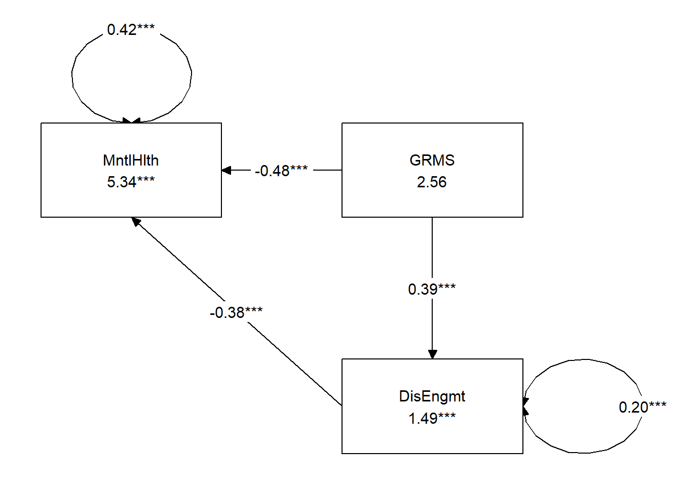 We can use the tidySEM::get_layout function to understand how our model is being mapped.
##      [,1]       [,2]
## [1,] NA         "GRMS"
## [2,] "MntlHlth" "DisEngmt"
## attr(,"class")
## [1] "layout_matrix" "matrix"        "array"
We can write code to remap them
##      [,1]   [,2]       [,3]
## [1,] ""     "DisEngmt" ""
## [2,] "GRMS" ""         "MntlHlth"
## attr(,"class")
## [1] "layout_matrix" "matrix"        "array"
We can update the tidySEM::graph_sem function with our new model to produce something that will better convey our analyses and its results.
tidySEM::graph_sem(LMed_fit, layout = Lmedmap, rect_width = 1.25, rect_height = 1.25,
    spacing_x = 2, spacing_y = 3, text_size = 4.5)
8.6 The Moderated Mediation: A Combined analysis
For a quick reminder, the diagram with labeled paths will help specify this in lavaan.
Looking at the diagram, with two consequent variables (i.e., those with arrows pointing to them) we can see two equations are needed to explain the model:
\[M = i_{M}+a_{1}X + a_{2}W + a_{3}XW + e_{M}\]
\[Y = i_{Y}+c_{1}^{'}X+ c_{2}^{'}W+c_{3}^{'}XW+ bM+e_{Y}\] Y = MntlHlth X = GRMS W = DisEngmt M = GRIcntlty
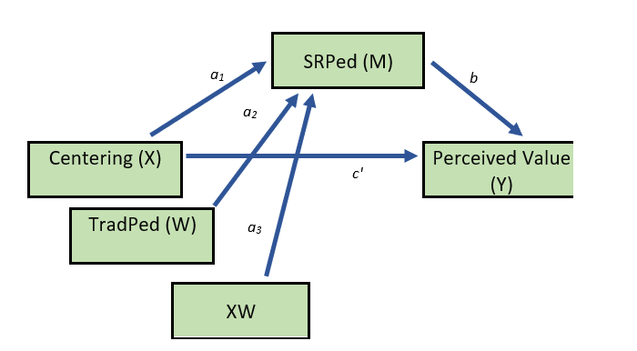
8.6.1 Specification in lavaan
In the code below
- First specify the equations, hints
- the a,b,c, labels are affixed with the *(asterisk)
- interaction terms are identifed with the colon
- Create code for the intercepts (Y and M) with the form: VarName ~ VarName.mean*1
- Create code for the mean and variance of all moderators (W, Z, etc.); these will be used in simple slopes.
- Means use the form: VarName ~ VarName.mean*1
- Variances use the form: VarName ~~VarName.var*VarName
- Calculate the index of moderated mediation: quantifies the relationship between the moderator and the indirect effect.
- To the degree that the value of the IMM is different from zero and the associated inferential test is statistically significant (bootstrapped confidence intervals are preferred; more powerful), we can conclude that the indirect effect is moderated.
- The IMM is used in the formula to calculate the conditional indirect effects.
- Hayes argues that a statistically significant IMM suggest they are (boom, done, p. 430).
- To the degree that the value of the IMM is different from zero and the associated inferential test is statistically significant (bootstrapped confidence intervals are preferred; more powerful), we can conclude that the indirect effect is moderated.
- Create code to calculate indirect effects conditional on (M +/- 1SD) moderator with the general form:
- product of the indirect effect (a*b) PLUS
- the product of the IMM and the moderated value
- Because our direct path is moderated, we will use a similar process to specify the direct effects conditional on (M +/- 1SD) moderator with the general form:
- the direct effect (c_p1) PLUS
- the moderated value (c_p3) at each of the three levels (M +/- 1SD)
- Although they don’t tend to be reported, you can create total effects conditional on the (M +/- 1SD). These are simply the sum of the c_p and all indirect paths, specified individually, at their M +/- 1SD conditional values.
Combined <- '
    #equations
    DisEngmt ~ a1*GRMS + a2*Centrality + a3*GRMS:Centrality
    MntlHlth ~ c_p1*GRMS + c_p2*Centrality + c_p3*GRMS:Centrality + b*DisEngmt

    #intercepts
    DisEngmt ~ DisEngmt.mean*1
    MntlHlth ~ MntlHlth.mean*1

    #means, variances of W for simple slopes
    Centrality ~ Centrality.mean*1
    Centrality ~~ Centrality.var*Centrality

    #index of moderated mediation, there will be an a and b path in the product
    #if the a and/or b path is moderated, select the label that represents the moderation

    imm := a3*b

    #Note that we first create the indirect product, then add to it the product of the imm and the W level
    indirect.SDbelow := a1*b + imm*(Centrality.mean - sqrt(Centrality.var))
    indirect.mean := a1*b + imm*(Centrality.mean)
    indirect.SDabove := a1*b + imm*(Centrality.mean + sqrt(Centrality.var))

    #direct effect is also moderated so calculate with c_p1 + c_p3
    direct.SDbelow := c_p1 + c_p3*(Centrality.mean - sqrt(Centrality.var))
    direct.Smean := c_p1 + c_p3*(Centrality.mean)
    direct.SDabove := c_p1 + c_p3*(Centrality.mean + sqrt(Centrality.var))

 '
set.seed(230925) #required for reproducible results because lavaan introduces randomness into the calculations
Combined_fit <- lavaan::sem(Combined, data = Lewis_df, se = "bootstrap", missing = 'fiml', bootstrap = 1000)
## Warning in lav_partable_vnames(FLAT, "ov.x", warn = TRUE): lavaan WARNING:
## model syntax contains variance/covariance/intercept formulas
## involving (an) exogenous variable(s): [Centrality]; These
## variables will now be treated as random introducing additional
## free parameters. If you wish to treat those variables as fixed,
## remove these formulas from the model syntax. Otherwise, consider
## adding the fixed.x = FALSE option.cFITsum <- lavaan::summary(Combined_fit, standardized = TRUE, rsq=T, ci=TRUE)
cParamEsts <- lavaan::parameterEstimates(Combined_fit, boot.ci.type = "bca.simple", standardized=TRUE)
cFITsum## lavaan 0.6.17 ended normally after 20 iterations
##
## Estimator ML
## Optimization method NLMINB
## Number of model parameters 13
##
## Number of observations 231
## Number of missing patterns 1
##
## Model Test User Model:
##
## Test statistic 567.225
## Degrees of freedom 2
## P-value (Chi-square) 0.000
##
## Parameter Estimates:
##
## Standard errors Bootstrap
## Number of requested bootstrap draws 1000
## Number of successful bootstrap draws 1000
##
## Regressions:
## Estimate Std.Err z-value P(>|z|) ci.lower ci.upper
## DisEngmt ~
## GRMS (a1) 0.623 0.194 3.212 0.001 0.166 0.942
## Cntrlty (a2) 0.093 0.137 0.680 0.497 -0.215 0.335
## GRMS:Cn (a3) -0.058 0.050 -1.142 0.253 -0.147 0.055
## MntlHlth ~
## GRMS (c_p1) -1.023 0.299 -3.417 0.001 -1.572 -0.389
## Cntrlty (c_p2) -0.317 0.190 -1.671 0.095 -0.669 0.070
## GRMS:Cn (c_p3) 0.136 0.074 1.841 0.066 -0.017 0.274
## DsEngmt (b) -0.362 0.091 -3.965 0.000 -0.530 -0.176
## Std.lv Std.all
##
## 0.623 0.846
## 0.093 0.133
## -0.058 -0.414
##
## -1.023 -0.846
## -0.317 -0.275
## 0.136 0.593
## -0.362 -0.220
##
## Intercepts:
## Estimate Std.Err z-value P(>|z|) ci.lower ci.upper
## .DsEngmt (DsE.) 1.107 0.521 2.126 0.034 0.276 2.325
## .MntlHlt (MnH.) 6.539 0.714 9.155 0.000 4.946 7.863
## Cntrlty (Cnt.) 3.938 0.049 79.569 0.000 3.836 4.035
## Std.lv Std.all
## 1.107 2.090
## 6.539 7.515
## 3.938 5.223
##
## Variances:
## Estimate Std.Err z-value P(>|z|) ci.lower ci.upper
## Cntrlty (Cnt.) 0.568 0.054 10.608 0.000 0.464 0.675
## .DsEngmt 0.194 0.016 12.001 0.000 0.160 0.224
## .MntlHlt 0.412 0.040 10.379 0.000 0.333 0.482
## Std.lv Std.all
## 0.568 1.000
## 0.194 0.692
## 0.412 0.545
##
## R-Square:
## Estimate
## DisEngmt 0.308
## MntlHlth 0.455
##
## Defined Parameters:
## Estimate Std.Err z-value P(>|z|) ci.lower ci.upper
## imm 0.021 0.020 1.064 0.287 -0.022 0.060
## indirect.SDblw -0.159 0.045 -3.574 0.000 -0.247 -0.075
## indirect.mean -0.143 0.040 -3.600 0.000 -0.219 -0.064
## indirect.SDabv -0.128 0.040 -3.163 0.002 -0.209 -0.050
## direct.SDbelow -0.591 0.089 -6.661 0.000 -0.750 -0.404
## direct.Smean -0.488 0.067 -7.251 0.000 -0.613 -0.356
## direct.SDabove -0.386 0.085 -4.521 0.000 -0.546 -0.216
## Std.lv Std.all
## 0.021 0.091
## -0.159 0.199
## -0.143 0.290
## -0.128 0.381
## -0.591 1.657
## -0.488 2.249
## -0.386 2.842## lhs op rhs
## 1 DisEngmt ~ GRMS
## 2 DisEngmt ~ Centrality
## 3 DisEngmt ~ GRMS:Centrality
## 4 MntlHlth ~ GRMS
## 5 MntlHlth ~ Centrality
## 6 MntlHlth ~ GRMS:Centrality
## 7 MntlHlth ~ DisEngmt
## 8 DisEngmt ~1
## 9 MntlHlth ~1
## 10 Centrality ~1
## 11 Centrality ~~ Centrality
## 12 DisEngmt ~~ DisEngmt
## 13 MntlHlth ~~ MntlHlth
## 14 GRMS ~~ GRMS
## 15 GRMS ~~ GRMS:Centrality
## 16 GRMS:Centrality ~~ GRMS:Centrality
## 17 GRMS ~1
## 18 GRMS:Centrality ~1
## 19 imm := a3*b
## 20 indirect.SDbelow := a1*b+imm*(Centrality.mean-sqrt(Centrality.var))
## 21 indirect.mean := a1*b+imm*(Centrality.mean)
## 22 indirect.SDabove := a1*b+imm*(Centrality.mean+sqrt(Centrality.var))
## 23 direct.SDbelow := c_p1+c_p3*(Centrality.mean-sqrt(Centrality.var))
## 24 direct.Smean := c_p1+c_p3*(Centrality.mean)
## 25 direct.SDabove := c_p1+c_p3*(Centrality.mean+sqrt(Centrality.var))
## label est se z pvalue ci.lower ci.upper std.lv std.all
## 1 a1 0.623 0.194 3.212 0.001 0.159 0.937 0.623 0.846
## 2 a2 0.093 0.137 0.680 0.497 -0.244 0.317 0.093 0.133
## 3 a3 -0.058 0.050 -1.142 0.253 -0.143 0.060 -0.058 -0.414
## 4 c_p1 -1.023 0.299 -3.417 0.001 -1.601 -0.420 -1.023 -0.846
## 5 c_p2 -0.317 0.190 -1.671 0.095 -0.669 0.070 -0.317 -0.275
## 6 c_p3 0.136 0.074 1.841 0.066 -0.009 0.281 0.136 0.593
## 7 b -0.362 0.091 -3.965 0.000 -0.527 -0.171 -0.362 -0.220
## 8 DisEngmt.mean 1.107 0.521 2.126 0.034 0.328 2.410 1.107 2.090
## 9 MntlHlth.mean 6.539 0.714 9.155 0.000 4.983 7.866 6.539 7.515
## 10 Centrality.mean 3.938 0.049 79.569 0.000 3.832 4.035 3.938 5.223
## 11 Centrality.var 0.568 0.054 10.608 0.000 0.469 0.682 0.568 1.000
## 12 0.194 0.016 12.001 0.000 0.166 0.235 0.194 0.692
## 13 0.412 0.040 10.379 0.000 0.345 0.510 0.412 0.545
## 14 0.518 0.000 NA NA 0.518 0.518 0.518 1.000
## 15 2.334 0.000 NA NA 2.334 2.334 2.334 0.853
## 16 14.446 0.000 NA NA 14.446 14.446 14.446 1.000
## 17 2.557 0.000 NA NA 2.557 2.557 2.557 3.552
## 18 10.199 0.000 NA NA 10.199 10.199 10.199 2.683
## 19 imm 0.021 0.020 1.064 0.287 -0.017 0.063 0.021 0.091
## 20 indirect.SDbelow -0.159 0.045 -3.574 0.000 -0.253 -0.083 -0.159 0.199
## 21 indirect.mean -0.143 0.040 -3.600 0.000 -0.226 -0.073 -0.143 0.290
## 22 indirect.SDabove -0.128 0.040 -3.163 0.002 -0.229 -0.061 -0.128 0.381
## 23 direct.SDbelow -0.591 0.089 -6.661 0.000 -0.754 -0.410 -0.591 1.657
## 24 direct.Smean -0.488 0.067 -7.251 0.000 -0.613 -0.355 -0.488 2.249
## 25 direct.SDabove -0.386 0.085 -4.521 0.000 -0.549 -0.218 -0.386 2.842
## std.nox
## 1 1.176
## 2 0.127
## 3 -0.109
## 4 -1.175
## 5 -0.262
## 6 0.156
## 7 -0.220
## 8 2.090
## 9 7.515
## 10 5.223
## 11 1.000
## 12 0.692
## 13 0.545
## 14 0.518
## 15 2.334
## 16 14.446
## 17 2.557
## 18 10.199
## 19 0.024
## 20 -0.158
## 21 -0.134
## 22 -0.110
## 23 -0.517
## 24 -0.361
## 25 -0.205# only worked when I used the library to turn on all these pkgs
library(lavaan)
library(dplyr)
library(ggplot2)
library(tidySEM)
tidySEM::graph_sem(model = Combined_fit)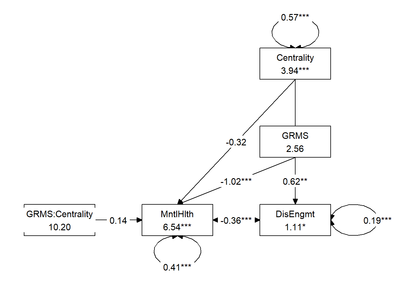 We can use the tidySEM::get_layout function to understand how our model is being mapped.
##      [,1]              [,2]         [,3]
## [1,] NA                "Centrality" "GRMS"
## [2,] "GRMS:Centrality" "MntlHlth"   "DisEngmt"
## attr(,"class")
## [1] "layout_matrix" "matrix"        "array"
We can write code to remap them
comb_map <- tidySEM::get_layout("", "DisEngmt", "", "GRMS", "", "MntlHlth",
    "Centrality", "", "", "", "GRMS:Centrality", "", rows = 4)
comb_map
## [,1] [,2] [,3]
## [1,] "" "DisEngmt" ""
## [2,] "GRMS" "" "MntlHlth"
## [3,] "Centrality" "" ""
## [4,] "" "GRMS:Centrality" ""
## attr(,"class")
## [1] "layout_matrix" "matrix" "array"We can update the tidySEM::graph_sem function with our new model to produce something that will better convey our analyses and its results.
tidySEM::graph_sem(Combined_fit, layout = comb_map, rect_width = 1.25,
    rect_height = 1.25, spacing_x = 2, spacing_y = 3, text_size = 3.5)
8.6.2 Beginning the interpretation
We have already looked at some of the simple effects found within the more complex model. Let’s grab the formulae.
\[\hat{M} = i_{M}+a_{1}X + a_{2}W + a_{3}XW + e_{M}\]
\[\hat{Y} = i_{Y}+c_{1}^{'}X+ c_{2}^{'}W+c_{3}^{'}XW+ bM+e_{Y}\]
And substitute in our values
\[\hat{M} = 1.417 + 0.212X + (-0.027) W + 0.006XW\] \[\hat{Y} = 31.703 + (-1.4115)X + (-0.556)W + 0.164XW + (-3.567)M\]
8.6.3 Tabling the data
Table 1
| Analysis of Moderated Mediation for GRMS, Gendered Racial Identity Centrality, Coping, and Mental Health |
|---|
| Predictor | \(B\) | \(SE_{B}\) | \(p\) | \(R^2\) |
|---|
| Disengagement coping (M) | .31 | |||
|---|---|---|---|---|
| Constant | 1.107 | 0.521 | 0.034 | |
| GRMS (\(a_1\)) | 0.623 | 0.194 | 0.001 | |
| Centrality (\(a_2\)) | 0.093 | 0.137 | 0.497 | |
| GRMS:Centrality (\(a_3\)) | -0.058 | 0.050 | 0.253 |
| Mental Health (DV) | .46 | |||
|---|---|---|---|---|
| Constant | 6.539 | 0.714 | <0.001 | |
| GRMS (\(c'_1\)) | -1.023 | 0.299 | 0.001 | |
| Centrality (\(c'_2\)) | -0.317 | 0.190 | 0.095 | |
| GRMS:Centrality (\(c'_3\)) | 0.136 | 0.074 | 0.066 | |
| Disengagement (\(b\)) | -0.362 | 0.091 | <0.001 |
| Summary of Effects | \(B\) | \(SE_{B}\) | \(p\) | 95% CI |
|---|---|---|---|---|
| IMM | 0.021 | 0.020 | 0.287 | -0.017, 0.063 |
| Indirect (\(-1SD\)) | -0.159 | 0.045 | <0.001 | -0.253, -0.083 |
| Indirect (\(M\)) | -0.143 | 0.040 | <0.001 | -0.226, -0.073 |
| Indirect (\(+1SD\)) | -0.128 | 0.040 | 0.002 | -0.229, -0.061 |
| Direct (\(-1SD\)) | -0.591 | 0.089 | <0.001 | -0.754, -0.410 |
| Direct (\(M\)) | -0.488 | 0.067 | <0.001 | -0.613, -0.355 |
| Direct (\(+1SD\)) | -0.386 | 0.085 | <0.001 | -0.549, -0.218 |
| Note. GRMS = gendered racial microaggressions. The significance of the indirect effects was calculated with bootstrapped, bias-corrected, confidence intervals (.95). |
Thirty one percent of the variance in disengagement coping (mediator) and 46% of the variance in mental health (DV) are predicted by their respective models.
The model we tested suggested that both the indirect and direct effects should be moderated.
8.6.3.1 Conditional Indirect effects
An indirect effect can be moderated if either the a or b path (or both) is(are) moderated. If at least one of the indirect paths is part of a moderation, then the whole indirect (axb) path would be moderated. In this model, we specified a moderation of the a path. We know the a path is moderated if the moderation term is statistically significant.
In our case, \(a_{3}\) GRMS:Centrality was not statistically significant \((B = -0.058, p = 0.253)\). We also inspect the Index of Moderated Mediation. The IMM is the product of the moderated path (in this case, the value of \(a_{3}\)) and b. If this index is 0, then the slope of the line for the indirect effect is flat. The bootstrap confidence interval associated with this test is the way to determine whether/not this slope is statistically significant from zero. In our case, IMM = 0.021 ($p = 0.287%) with the 95% confidence interval ranging from CI095 = -0.017 to 0.063. This suggests that we do not have a moderated mediation. Hayes claims the IMM saves us from formally comparing (think “contrasts” pairs of conditional indirect effects).
We can obtain more information about the potentially moderated indirect effect by probing the conditional indirect effect. Because an indirect effect is not normally distributed, Hayes discourages using a Johnson-Neyman approach and suggests that we use a pick-a-point. He usually selects the 16th, 50th, and 84th percentiles of the distribution. However, many researchers commonly report the mean+/-1SD.
- at 1SD below the mean \(B = -0.159, p <0.001, 95CI(-0.253, -0.083)\);
- at the mean \(B = -0.488, p <0.001, 95CI(-0.613, -0.355)\);
- at 1SD above the mean, \(B = -0.128, p = 0.002, 95CI(-0.229, -0.061)\).
Examining the relative consistency of the \(B\) weights and the consistently significant \(p\) values, we see that there was an indirect effect throughout the varying levels of the moderator, gendered racial identity centrality. Thus, it makes sense that this was not a moderated mediation.
8.6.3.2 Conditional Direct effect
The direct effect of X to Y estimates how differences in X relate to differences in Y holding constant the proposed mediator(s). We know the direct effect is moderated if the interaction term \((c'_p3)\)is statistically significant. In our case, it was not \(B = 0.136, p = 0.066\). Probing a conditional direct effect is straightforward – we typically use the same points as we did in the probing of the conditional indirect effect.
- at 1SD below the mean \(B = -0.591, p <0.001, 95CI(-0.754, -0.410)\);
- at the mean \(B-0.143, p <0.001, 95CI(-0.226, -0.073)\);
- at 1SD above the mean, \(B = -0.386, p <0.001, 95CI(-0.549, -0.218)\).
The statistically significant effect of GRMS on mental health at the three levels of gendered racial identity centrality is consistent with the non-significant interaction effect.
8.6.4 Model trimming
Hayes terms it pruning when he suggests that when there is no moderation of an effect, the researcher may want to delete that interaction term. In our case, neither the direct nor indirect effect was moderated (although the +1SD was close (\(B = 0.136, p = 0.066\)). Deleting these paths one at a time is typical practice because the small boost of power with each deleted path may “turn on” significance elsewhere. If I were to engage in model trimming, I would start with the indirect effect to see if the interaction term associated with the direct effect became statistically significant. This is consistent with the simple moderation we ran earlier where we saw a fanning out at one end of the distribution.
8.6.5 APA Style Write-up
As we look to write up our own results I encourage you to review the manuscript that sources our research vignette. The Lewis et al. (2017) write-up is an efficient one, simultaneously presenting the results of two outcome variables – mental and physical health. While our B weights from our simulated data map similarly onto those reported in the Lewis et al. manuscript, we do not get get the statistically significant moderated mediation reported in the article.
Method/Analytic Strategy
Data were analyzed with a maximum likelihood approach the package, lavaan (v. 0.6-16). We specified a moderated mediation model predicting mental health from gendered racial microaggressions, mediated by disengagement coping. We further predicted that the relationships between gendered racial microaggressions to disengagement coping (i.e., the a path) and between gendered racial microaggressions to mental health (i.e., the \(c^1\) path) would be moderated by gendered racial identity centrality.
Results
Preliminary Analyses
- Missing data analysis and managing missing data
- Bivariate correlations, means, SDs
- Distributional characteristics, assumptions, etc.
- Address limitations and concerns
Primary Analyses Our analysis evaluated a moderation mediation model predicting mental health (Y/MntlHlth) from gendered racial microaggressions (X/GRMS) mediated by disengagement coping (M/DisEngmt). Gendered racial identity centrality (W/GRIcntrlty) was our moderating variable. We specified a moderation of path a (X/GRMS to M/DisEngmt) and the direct path, c’ (X/GRMS to Y/MntlHlth). Data were analyzed with maximum likelihood estimation in the R package lavaan (v. 0.6-7); the significance of effects were tested with 1000 bootstrap confidence intervals. Results of the full model are presented in Table 1 and illustrated in Figure 1 (a variation of the semPlot or Hayes style representation). The formula for the mediator and dependent variable are expressed below.
\[\hat{M} = 1.107 + 0.623X + (0.093) W + -0.058XW\] \[\hat{Y} = 6.539 + (-1.023)X + (-0.317)W +0.136XW + (-0.362)M\]
Results suggested a negative effect of gendered racial microaggressions on mental health that is mediated through disengagement coping. That is, in the presence of gendered racial microaggressions, participants increased disengagement coping which, in turn, had negative effects on mental health. The index of moderated mediation was not significant \((B = 0.021, p = 0.287, 95CI(-0.017, 0.063)\), suggesting that the indirect effects were not conditional on the values of the moderator. While there was no evidence of moderation on the indirect or direct paths, there was a statistically significant, and consistently strong, mediation throughout the range of the gendered racial identity centrality (moderator). Because we did not have a moderated mediation, I would probably not include the rest of this paragraph (nor include the moderation figure). I just wanted to demonstrate how to talk about findings if they were significant (although I acnowledg throughat that these are non-significant). Figure 2 illustrates the conditional effects (non-significant) of GRMS (X) on mental health (Y) among those at the traditional levels of \(M \pm 1SD\). Our model accounted for 31% of the variance in the mediator (disengagement coping) and 46% of the variance in the dependent variable (mental health).

8.7 STAY TUNED
A section on power analysis is planned and coming soon! My apologies that it’s not quite Ready.
8.9 Practice Problems
The three problems described below were designed to grow during the series of chapters on simple and complex mediation, complex moderation, and conditional process analysis (i.e,. this chapter). I have recommended that you select a dataset that includes at least four variables. If you are new to this topic, you may wish to select variables that are all continuously scaled. The IV and moderator (next chapters) could be categorical (if they are dichotomous, please use 0/1 coding; if they have more than one category it is best if they are ordered). You will likely encounter challenges that were not covered in this chapter. Search for and try out solutions, knowing that there are multiple paths through the analysis.
The suggested practice problem for this chapter is to conduct a moderated mediation. At least one path (a or b) should be moderated.
8.9.1 Problem #1: Rework the research vignette as demonstrated, but change the random seed
If this topic feels a bit overwhelming, simply change the random seed in the data simulation, then rework the problem. This should provide minor changes to the data (maybe in the second or third decimal point), but the results will likely be very similar.
8.9.2 Problem #2: Rework the research vignette, but swap one or more variables
Use the simulated data, but select one of the other models that was evaluated in the Lewis et al. (2017) study. For example, physical health was also used as a dependent variable in a separate but otherwise parallel analysis. Compare your results to those reported in the mansucript.
8.9.3 Problem #3: Use other data that is available to you
Using data for which you have permission and access (e.g., IRB approved data you have collected or from your lab; data you simulate from a published article; data from an open science repository; data from other chapters in this OER), complete a simple mediation.
8.9.4 Grading Rubric
| Assignment Component | ||
|---|---|---|
| 1. Describing the overall model hypothesis, assign each variable to the X, Y, M, or W roles | 5 | _____ |
| 2. Import and format the variables in the model | 5 | _____ |
| 3. Using a piecewise approach, run each of the simple models in the grander design | 5 | _____ |
| 4. Specify and run the entire lavaan model | 5 | _____ |
| 5. Use tidySEM to create a figure | 5 | _____ |
| 6. Create a table that includes regression output for the M and Y variables and the moderated effects | 5 | _____ |
| 7. Represent your work in an APA-style write-up | 5 | _____ |
| 8. Explanation to grader | 5 | _____ |
| 9. Be able to hand-calculate the indirect, direct, and total effects from the a, b, & c’ paths | 5 | _____ |
| Totals | 45 | _____ |
8.10 Homeworked Example 1: A moderation on the a path
For more information about the data used in this homeworked example, please refer to the description and codebook located at the end of the introductory lesson in ReCentering Psych Stats. An .rds file which holds the data is located in the Worked Examples folder at the GitHub site the hosts the OER. The file name is ReC.rds.
The suggested practice problem for this chapter is to conduct a moderated mediation. At least one path (a or b) should be moderated.
Describing thy overall model hypothesis, assign each variable to the X, Y, M, and W roles
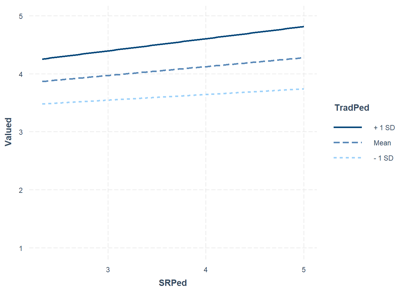
My analysis will evaluated a moderated mediation. Specifically, I predict that the effect of centering on perceived value to the student will be moderated by the students’ evaluation of socially responsive pedagogy. I further hypothesize that this indirect effect will be moderated by traditional pedagogy and that the moderation will occur on the a path, that is, traditional pedagogy will moderate the effect of centering on socially responsive pedagogy.
- X = Centering, pre/re (0,1)
- W = Traditional Pedagogy (1 to 4 scaling)
- M = Socially Responsive Pedagogy (1 to 4 scaling)
- Y = Value to the student (1 to 4 scaling)
Import the data and format the variables in the model
The approach we are taking to moderated mediation does not allow dependency in the data. Therefore, we will include only those who took the multivariate class (i.e., excluding responses for the ANOVA and psychometrics courses).
I need to score the SRPed, TradPed, and Valued variables
TradPed_vars <- c("ClearResponsibilities", "EffectiveAnswers", "Feedback",
    "ClearOrganization", "ClearPresentation")
raw$TradPed <- sjstats::mean_n(raw[, ..TradPed_vars], 0.75)

Valued_vars <- c("ValObjectives", "IncrUnderstanding", "IncrInterest")
raw$Valued <- sjstats::mean_n(raw[, ..Valued_vars], 0.75)

SRPed_vars <- c("InclusvClassrm", "EquitableEval", "MultPerspectives",
    "DEIintegration")
raw$SRPed <- sjstats::mean_n(raw[, ..SRPed_vars], 0.75)
I will create a babydf.
Let’s check the structure of the variables:
## Classes 'data.table' and 'data.frame':   84 obs. of  4 variables:
##  $ Centering: Factor w/ 2 levels "Pre","Re": 2 2 2 2 2 2 2 2 2 2 ...
##  $ TradPed  : num  3.8 5 4.8 4 4.2 3 5 4.6 4 4.8 ...
##  $ SRPed    : num  4.5 5 5 5 4.75 4.5 5 4.5 5 5 ...
##  $ Valued   : num  4.33 5 4.67 3.33 4 3.67 5 4 4.67 4.67 ...
##  - attr(*, ".internal.selfref")=<externalptr>
In later analyses, it will be important that Centering is a dummy-coded numerical variable:
babydf$CENTERING <- as.numeric(babydf$Centering)
babydf$CENTERING <- (babydf$CENTERING - 1)
str(babydf)
## Classes 'data.table' and 'data.frame': 84 obs. of 5 variables:
## $ Centering: Factor w/ 2 levels "Pre","Re": 2 2 2 2 2 2 2 2 2 2 ...
## $ TradPed : num 3.8 5 4.8 4 4.2 3 5 4.6 4 4.8 ...
## $ SRPed : num 4.5 5 5 5 4.75 4.5 5 4.5 5 5 ...
## $ Valued : num 4.33 5 4.67 3.33 4 3.67 5 4 4.67 4.67 ...
## $ CENTERING: num 1 1 1 1 1 1 1 1 1 1 ...
## - attr(*, ".internal.selfref")=<externalptr>Quick peek at relations between variables:
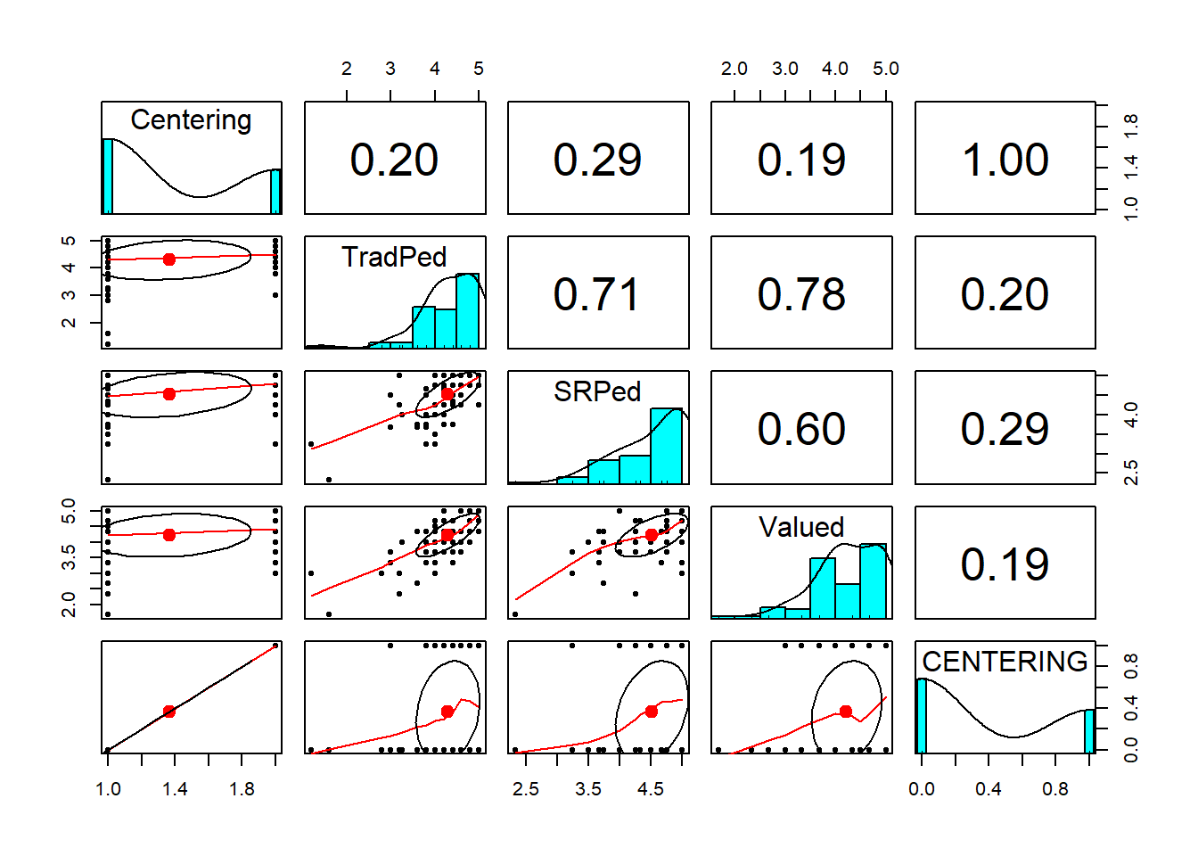
Using a piecewise approach, run each of the simple models in the grander design
Analysis #1: A simple moderation of the a path
We are asking, “Does traditional pedagogy moderate the relationship between centering and socially responsive pedagogy?
Y = socially responsive pedagogy X = centering W = traditional pedagogy
Let’s specify this simple moderation model with base R’s lm() function.
mod_a_path <- lm(SRPed ~ Centering * TradPed, data = babydf)
# the base R output if you prefer this view
summary(mod_a_path)
##
## Call:
## lm(formula = SRPed ~ Centering * TradPed, data = babydf)
##
## Residuals:
## Min 1Q Median 3Q Max
## -1.30064 -0.24549 0.07396 0.15007 1.21341
##
## Coefficients:
## Estimate Std. Error t value Pr(>|t|)
## (Intercept) 1.89621 0.30253 6.268 0.00000001948738 ***
## CenteringRe 1.15285 0.73720 1.564 0.122
## TradPed 0.59074 0.07064 8.362 0.00000000000204 ***
## CenteringRe:TradPed -0.21535 0.16486 -1.306 0.195
## ---
## Signif. codes: 0 '***' 0.001 '**' 0.01 '*' 0.05 '.' 0.1 ' ' 1
##
## Residual standard error: 0.399 on 77 degrees of freedom
## (3 observations deleted due to missingness)
## Multiple R-squared: 0.5413, Adjusted R-squared: 0.5235
## F-statistic: 30.29 on 3 and 77 DF, p-value: 0.0000000000004875We’ll use the jtools package so we get that great summ function and interactions for the awesome plot.
Since we are just working to understand our moderations, we can run them with “regular old” ordinary least squares.
# library(jtools) #the summ function creates a terrific regression
# table library(interactions)
library(ggplot2)

jtools::summ(mod_a_path, digits = 3)| Observations | 81 (3 missing obs. deleted) |
| Dependent variable | SRPed |
| Type | OLS linear regression |
| F(3,77) | 30.294 |
| R² | 0.541 |
| Adj. R² | 0.523 |
| Est. | S.E. | t val. | p | |
|---|---|---|---|---|
| (Intercept) | 1.896 | 0.303 | 6.268 | 0.000 |
| CenteringRe | 1.153 | 0.737 | 1.564 | 0.122 |
| TradPed | 0.591 | 0.071 | 8.362 | 0.000 |
| CenteringRe:TradPed | -0.215 | 0.165 | -1.306 | 0.195 |
| Standard errors: OLS |
Looking at these results we can see that the predictors account for about 54% of variance in perceived value to the student. Only the moderator (TradPed, W), traditional pedagogy is a significant predictor. Neither the independent variable (Centering, X), nor its interaction with Centering (Centering:TradPed, XW) are significant.
It’s always helpful to graph the relationship. The interaction_plot() function from the package, interactions can make helpful illustrations. In the case of interactions/moderations, I like to run them “both ways” to see which makes more sense.

## Warning: Johnson-Neyman intervals are not available for factor moderators.## SIMPLE SLOPES ANALYSIS
##
## Slope of TradPed when Centering = Re:
##
## Est. S.E. t val. p
## ------ ------ -------- ------
## 0.38 0.15 2.52 0.01
##
## Slope of TradPed when Centering = Pre:
##
## Est. S.E. t val. p
## ------ ------ -------- ------
## 0.59 0.07 8.36 0.00# sim_slopes(Mod_a_path, pred=GRIcntlty, modx = GRMS) #sometimes I
# like to look at it in reverse -- like in the plotsConsistent with the non-signicant interation effect but the significant main effect, there was a statistically significant effect of traditional pedagogy on socially responsive pedagogy for both pre-centered and re-centered stages.
Traditional pedagogy is the only significant predictor in socially responsive pedagogy. Overall, the model accounts for 54% of the variance in socially responsive pedagogy.
Analysis #2: A simple mediation
We are asking, “Does socially responsive pedagogy mediate the relationship between centering and perceived value to the student?”
Y = perceived value X = centering M = socially responsive pedagogy
Note. I switched to using the CENTERING (all caps) variable because it is 0/1, numeric (better for lavaan).
library(lavaan)

medmodel <- "
          Valued ~ b*SRPed + c_p*CENTERING
          SRPed ~a*CENTERING

          #intercepts
          CENTERING ~ CENTERING.mean*1
          Valued ~ Valued.mean*1

          indirect :=  a*b
          direct  := c_p
          total_c  := c_p + (a*b)
          "
set.seed(230925)  #required for reproducible results because lavaan introduces randomness into the calculations
medmodel_fit <- lavaan::sem(medmodel, data = babydf, se = "bootstrap",
    missing = "fiml")
medmodel_Sum <- lavaan::summary(medmodel_fit, standardized = T, rsq = T,
    ci = TRUE)
medmodel_ParEsts <- lavaan::parameterEstimates(medmodel_fit, boot.ci.type = "bca.simple",
    standardized = TRUE)
medmodel_Sum
## lavaan 0.6.17 ended normally after 25 iterations
##
## Estimator ML
## Optimization method NLMINB
## Number of model parameters 9
##
## Number of observations 84
## Number of missing patterns 2
##
## Model Test User Model:
##
## Test statistic 0.000
## Degrees of freedom 0
##
## Parameter Estimates:
##
## Standard errors Bootstrap
## Number of requested bootstrap draws 1000
## Number of successful bootstrap draws 1000
##
## Regressions:
## Estimate Std.Err z-value P(>|z|) ci.lower ci.upper
## Valued ~
## SRPed (b) 0.728 0.124 5.877 0.000 0.455 0.933
## CENTERIN (c_p) 0.004 0.124 0.032 0.974 -0.225 0.257
## SRPed ~
## CENTERIN (a) 0.367 0.114 3.225 0.001 0.148 0.601
## Std.lv Std.all
##
## 0.728 0.608
## 0.004 0.003
##
## 0.367 0.307
##
## Intercepts:
## Estimate Std.Err z-value P(>|z|) ci.lower ci.upper
## CENTERI (CENT) 0.369 0.054 6.872 0.000 0.274 0.476
## .Valued (Vld.) 0.935 0.548 1.707 0.088 0.018 2.136
## .SRPed 4.371 0.086 50.597 0.000 4.187 4.527
## Std.lv Std.all
## 0.369 0.765
## 0.935 1.355
## 4.371 7.580
##
## Variances:
## Estimate Std.Err z-value P(>|z|) ci.lower ci.upper
## .Valued 0.299 0.055 5.453 0.000 0.186 0.408
## .SRPed 0.301 0.058 5.157 0.000 0.196 0.413
## CENTERING 0.233 0.014 16.390 0.000 0.199 0.249
## Std.lv Std.all
## 0.299 0.629
## 0.301 0.906
## 0.233 1.000
##
## R-Square:
## Estimate
## Valued 0.371
## SRPed 0.094
##
## Defined Parameters:
## Estimate Std.Err z-value P(>|z|) ci.lower ci.upper
## indirect 0.267 0.100 2.665 0.008 0.095 0.488
## direct 0.004 0.124 0.032 0.974 -0.225 0.257
## total_c 0.271 0.144 1.886 0.059 -0.014 0.551
## Std.lv Std.all
## 0.267 0.187
## 0.004 0.003
## 0.271 0.190## lhs op rhs label est se z pvalue ci.lower
## 1 Valued ~ SRPed b 0.728 0.124 5.877 0.000 0.464
## 2 Valued ~ CENTERING c_p 0.004 0.124 0.032 0.974 -0.225
## 3 SRPed ~ CENTERING a 0.367 0.114 3.225 0.001 0.131
## 4 CENTERING ~1 CENTERING.mean 0.369 0.054 6.872 0.000 0.262
## 5 Valued ~1 Valued.mean 0.935 0.548 1.707 0.088 -0.040
## 6 Valued ~~ Valued 0.299 0.055 5.453 0.000 0.213
## 7 SRPed ~~ SRPed 0.301 0.058 5.157 0.000 0.205
## 8 CENTERING ~~ CENTERING 0.233 0.014 16.390 0.000 0.199
## 9 SRPed ~1 4.371 0.086 50.597 0.000 4.189
## 10 indirect := a*b indirect 0.267 0.100 2.665 0.008 0.109
## 11 direct := c_p direct 0.004 0.124 0.032 0.974 -0.225
## 12 total_c := c_p+(a*b) total_c 0.271 0.144 1.886 0.059 -0.025
## ci.upper std.lv std.all std.nox
## 1 0.939 0.728 0.608 0.608
## 2 0.250 0.004 0.003 0.003
## 3 0.587 0.367 0.307 0.307
## 4 0.476 0.369 0.765 0.765
## 5 2.084 0.935 1.355 1.355
## 6 0.454 0.299 0.629 0.629
## 7 0.424 0.301 0.906 0.906
## 8 0.249 0.233 1.000 1.000
## 9 4.528 4.371 7.580 7.580
## 10 0.528 0.267 0.187 0.187
## 11 0.250 0.004 0.003 0.003
## 12 0.546 0.271 0.190 0.190Our model accounts for 9% of the variance in socially responsive pedagogy and 37% of the variance in perceived value to the student. The a path (Centering –> SRPed), b path (SRPed –> Valued), and indirect effect are all statistically significant.
# only worked when I used the library to turn on all these pkgs
library(lavaan)
library(dplyr)
library(ggplot2)
library(tidySEM)
tidySEM::graph_sem(model = medmodel_fit)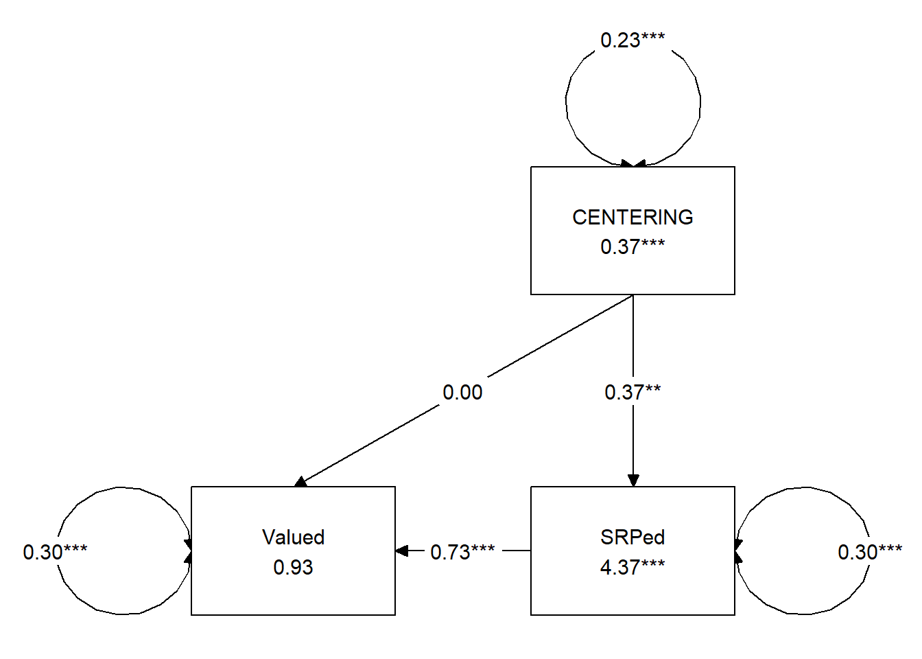
We can use the tidySEM::get_layout function to understand how our model is being mapped.
##      [,1]        [,2]
## [1,] "CENTERING" NA
## [2,] "SRPed"     "Valued"
## attr(,"class")
## [1] "layout_matrix" "matrix"        "array"
We can write code to remap them
##      [,1]        [,2]    [,3]
## [1,] ""          "SRPed" ""
## [2,] "CENTERING" ""      "Valued"
## attr(,"class")
## [1] "layout_matrix" "matrix"        "array"
We can update the tidySEM::graph_sem function with our new model to produce something that will better convey our analyses and its results.
tidySEM::graph_sem(medmodel_fit, layout = medmap, rect_width = 1.25, rect_height = 1.25,
spacing_x = 2, spacing_y = 3, text_size = 4.5)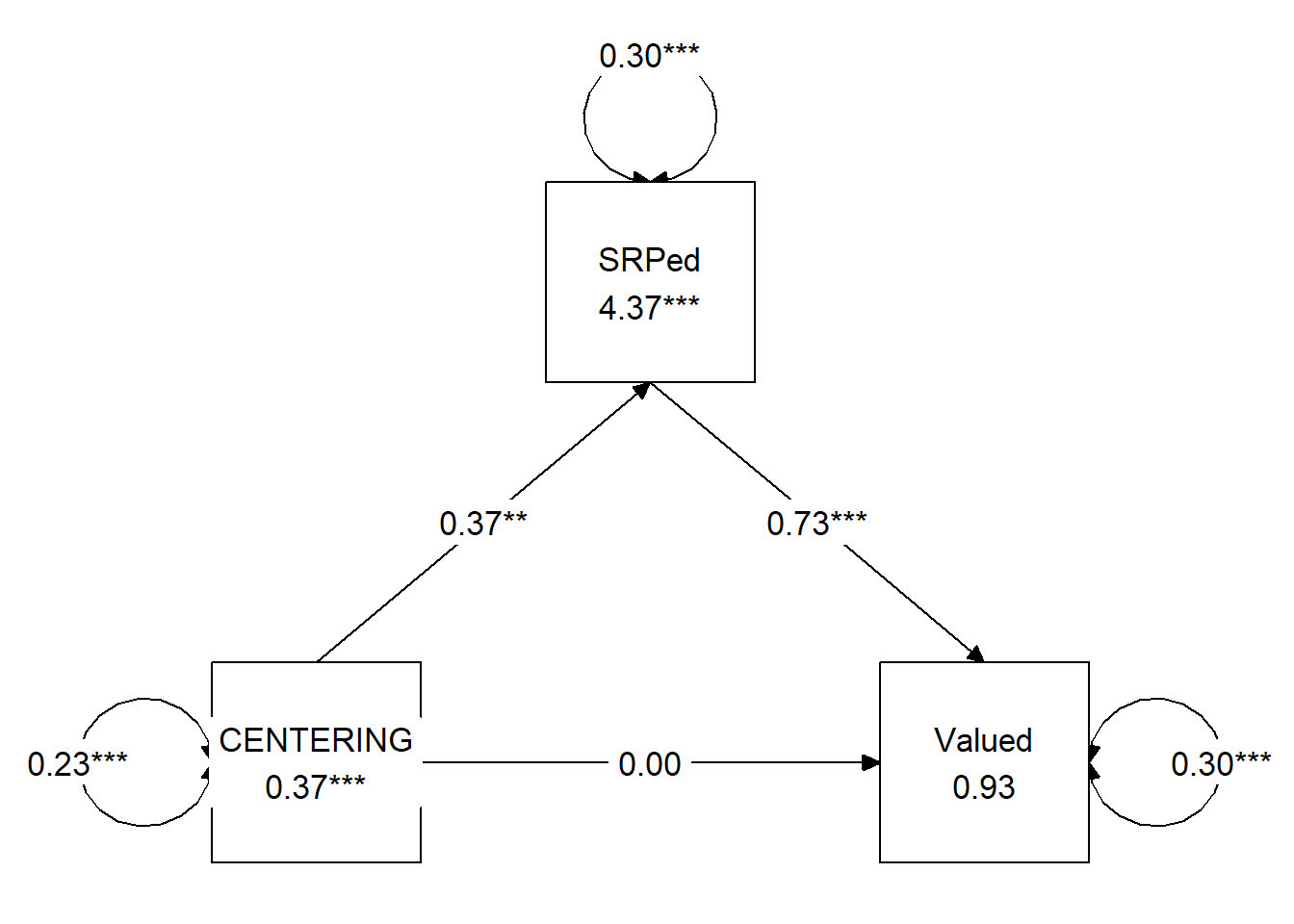 ### Specify and run the entire lavaan model {-}
set.seed(230925)
ModMedOnA <- "
    #equations
    SRPed ~ a1*CENTERING + a2*TradPed + a3*CENTERING:TradPed
    Valued ~ c_p*CENTERING + b*SRPed

    #intercepts
    SRPed ~ SRPed.mean*1
    Valued ~ Valued.mean*1

    #means, variances of W for simple slopes
    TradPed ~ TradPed.mean*1
    TradPed ~~ TradPed.var*TradPed

    #index of moderated mediation, there will be an a and b path in the product
    #if the a and/or b path is moderated, select the label that represents the moderation

    imm := a3*b

    #Note that we first create the indirect product, then add to it the product of the imm and the W level
    indirect.SDbelow := a1*b + imm*(TradPed.mean - sqrt(TradPed.var))
    indirect.mean := a1*b + imm*(TradPed.mean)
    indirect.SDabove := a1*b + imm*(TradPed.mean + sqrt(TradPed.var))

 "
set.seed(230925)  #required for reproducible results because lavaan introduces randomness into the calculations
ModMedOnA_fit <- lavaan::sem(ModMedOnA, data = babydf, se = "bootstrap",
    missing = "fiml", bootstrap = 1000)
## Warning in lav_data_full(data = data, group = group, cluster = cluster, : lavaan WARNING: 1 cases were deleted due to missing values in
## exogenous variable(s), while fixed.x = TRUE.## Warning in lav_partable_vnames(FLAT, "ov.x", warn = TRUE): lavaan WARNING:
## model syntax contains variance/covariance/intercept formulas
## involving (an) exogenous variable(s): [TradPed]; These variables
## will now be treated as random introducing additional free
## parameters. If you wish to treat those variables as fixed, remove
## these formulas from the model syntax. Otherwise, consider adding
## the fixed.x = FALSE option.ModMedOnAsum <- lavaan::summary(ModMedOnA_fit, standardized = TRUE, rsq = T,
ci = TRUE)
ModMedOnAParamEsts <- lavaan::parameterEstimates(ModMedOnA_fit, boot.ci.type = "bca.simple",
standardized = TRUE)
ModMedOnAsum## lavaan 0.6.17 ended normally after 36 iterations
##
## Estimator ML
## Optimization method NLMINB
## Number of model parameters 11
##
## Used Total
## Number of observations 83 84
## Number of missing patterns 2
##
## Model Test User Model:
##
## Test statistic 60.195
## Degrees of freedom 4
## P-value (Chi-square) 0.000
##
## Parameter Estimates:
##
## Standard errors Bootstrap
## Number of requested bootstrap draws 1000
## Number of successful bootstrap draws 1000
##
## Regressions:
## Estimate Std.Err z-value P(>|z|) ci.lower ci.upper
## SRPed ~
## CENTERIN (a1) 1.184 0.915 1.295 0.195 -1.022 2.719
## TradPed (a2) 0.597 0.095 6.304 0.000 0.451 0.819
## CENTERIN (a3) -0.222 0.194 -1.143 0.253 -0.543 0.246
## Valued ~
## CENTERIN (c_p) -0.011 0.122 -0.094 0.925 -0.234 0.243
## SRPed (b) 0.737 0.119 6.189 0.000 0.481 0.939
## Std.lv Std.all
##
## 1.184 0.965
## 0.597 0.728
## -0.222 -0.819
##
## -0.011 -0.008
## 0.737 0.625
##
## Intercepts:
## Estimate Std.Err z-value P(>|z|) ci.lower ci.upper
## .SRPed (SRP.) 1.865 0.433 4.308 0.000 0.826 2.538
## .Valued (Vld.) 0.900 0.527 1.708 0.088 -0.011 2.024
## TradPed (TrP.) 4.292 0.078 55.116 0.000 4.130 4.443
## Std.lv Std.all
## 1.865 3.164
## 0.900 1.294
## 4.292 5.977
##
## Variances:
## Estimate Std.Err z-value P(>|z|) ci.lower ci.upper
## TradPed (TrP.) 0.516 0.142 3.627 0.000 0.263 0.839
## .SRPed 0.151 0.029 5.119 0.000 0.089 0.206
## .Valued 0.296 0.054 5.489 0.000 0.182 0.399
## Std.lv Std.all
## 0.516 1.000
## 0.151 0.434
## 0.296 0.611
##
## R-Square:
## Estimate
## SRPed 0.566
## Valued 0.389
##
## Defined Parameters:
## Estimate Std.Err z-value P(>|z|) ci.lower ci.upper
## imm -0.164 0.144 -1.136 0.256 -0.416 0.185
## indirect.SDblw 0.288 0.177 1.625 0.104 -0.107 0.602
## indirect.mean 0.171 0.085 2.002 0.045 0.000 0.337
## indirect.SDabv 0.053 0.073 0.730 0.465 -0.093 0.190
## Std.lv Std.all
## -0.164 -0.512
## 0.288 -1.944
## 0.171 -2.456
## 0.053 -2.967## lhs op rhs
## 1 SRPed ~ CENTERING
## 2 SRPed ~ TradPed
## 3 SRPed ~ CENTERING:TradPed
## 4 Valued ~ CENTERING
## 5 Valued ~ SRPed
## 6 SRPed ~1
## 7 Valued ~1
## 8 TradPed ~1
## 9 TradPed ~~ TradPed
## 10 SRPed ~~ SRPed
## 11 Valued ~~ Valued
## 12 CENTERING ~~ CENTERING
## 13 CENTERING ~~ CENTERING:TradPed
## 14 CENTERING:TradPed ~~ CENTERING:TradPed
## 15 CENTERING ~1
## 16 CENTERING:TradPed ~1
## 17 imm := a3*b
## 18 indirect.SDbelow := a1*b+imm*(TradPed.mean-sqrt(TradPed.var))
## 19 indirect.mean := a1*b+imm*(TradPed.mean)
## 20 indirect.SDabove := a1*b+imm*(TradPed.mean+sqrt(TradPed.var))
## label est se z pvalue ci.lower ci.upper std.lv std.all
## 1 a1 1.184 0.915 1.295 0.195 -1.175 2.630 1.184 0.965
## 2 a2 0.597 0.095 6.304 0.000 0.448 0.806 0.597 0.728
## 3 a3 -0.222 0.194 -1.143 0.253 -0.523 0.287 -0.222 -0.819
## 4 c_p -0.011 0.122 -0.094 0.925 -0.236 0.237 -0.011 -0.008
## 5 b 0.737 0.119 6.189 0.000 0.487 0.946 0.737 0.625
## 6 SRPed.mean 1.865 0.433 4.308 0.000 0.894 2.551 1.865 3.164
## 7 Valued.mean 0.900 0.527 1.708 0.088 -0.027 1.985 0.900 1.294
## 8 TradPed.mean 4.292 0.078 55.116 0.000 4.129 4.434 4.292 5.977
## 9 TradPed.var 0.516 0.142 3.627 0.000 0.272 0.850 0.516 1.000
## 10 0.151 0.029 5.119 0.000 0.103 0.219 0.151 0.434
## 11 0.296 0.054 5.489 0.000 0.203 0.425 0.296 0.611
## 12 0.231 0.000 NA NA 0.231 0.231 0.231 1.000
## 13 1.036 0.000 NA NA 1.036 1.036 1.036 0.991
## 14 4.733 0.000 NA NA 4.733 4.733 4.733 1.000
## 15 0.361 0.000 NA NA 0.361 0.361 0.361 0.752
## 16 1.622 0.000 NA NA 1.622 1.622 1.622 0.745
## 17 imm -0.164 0.144 -1.136 0.256 -0.411 0.196 -0.164 -0.512
## 18 indirect.SDbelow 0.288 0.177 1.625 0.104 -0.096 0.631 0.288 -1.944
## 19 indirect.mean 0.171 0.085 2.002 0.045 0.013 0.361 0.171 -2.456
## 20 indirect.SDabove 0.053 0.073 0.730 0.465 -0.100 0.184 0.053 -2.967
## std.nox
## 1 2.010
## 2 0.487
## 3 -0.377
## 4 -0.016
## 5 0.625
## 6 3.164
## 7 1.294
## 8 5.977
## 9 1.000
## 10 0.434
## 11 0.611
## 12 0.231
## 13 1.036
## 14 4.733
## 15 0.361
## 16 1.622
## 17 -0.235
## 18 0.084
## 19 -0.151
## 20 -0.386Use tidySEM to create a figure
# only worked when I used the library to turn on all these pkgs
library(lavaan)
library(dplyr)
library(ggplot2)
library(tidySEM)
tidySEM::graph_sem(model = ModMedOnA_fit)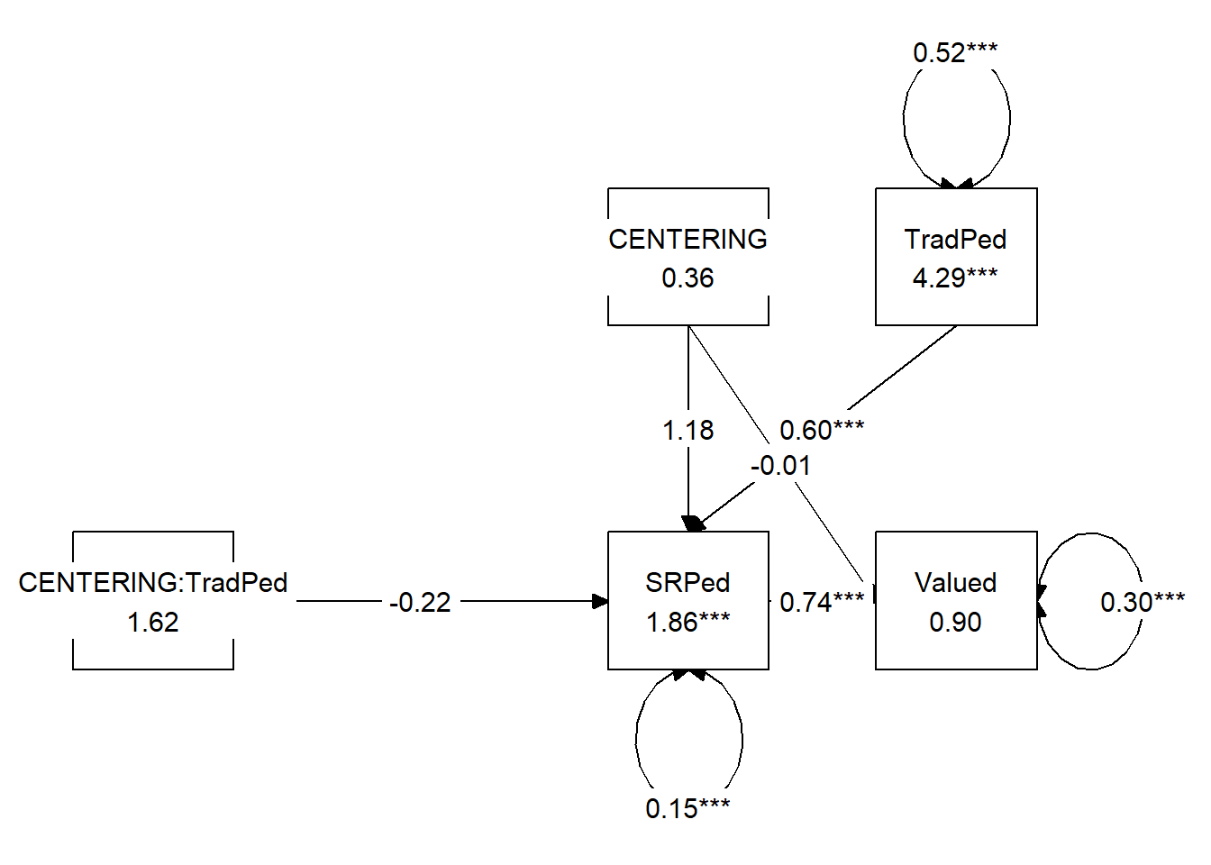
We can use the tidySEM::get_layout function to understand how our model is being mapped.
##      [,1]     [,2]                [,3]        [,4]
## [1,] NA       "CENTERING:TradPed" NA          NA
## [2,] NA       NA                  NA          NA
## [3,] "Valued" "SRPed"             "CENTERING" "TradPed"
## attr(,"class")
## [1] "layout_matrix" "matrix"        "array"
We can write code to remap them
comb_map <- tidySEM::get_layout("", "SRPed", "", "CENTERING", "", "Valued",
    "TradPed", "", "", "", "CENTERING:TradPed", "", rows = 4)
comb_map
## [,1] [,2] [,3]
## [1,] "" "SRPed" ""
## [2,] "CENTERING" "" "Valued"
## [3,] "TradPed" "" ""
## [4,] "" "CENTERING:TradPed" ""
## attr(,"class")
## [1] "layout_matrix" "matrix" "array"We can update the tidySEM::graph_sem function with our new model to produce something that will better convey our analyses and its results.
tidySEM::graph_sem(ModMedOnA_fit, layout = comb_map, rect_width = 1.5,
    rect_height = 1.25, spacing_x = 2, spacing_y = 3, text_size = 3.5)
Create a table that includes regression output for the M and Y variables and the moderated effects
Exporting the results to a .csv file will help us create a journal-ready table, outside of the R environment.
Table 1
| Analysis of Moderated Mediation for Centering, Socially Responsive Pedagogy, Traditional Pedagogy, and Perceived Value to the Student |
|---|
| Predictor | \(B\) | \(SE_{B}\) | \(p\) | \(R^2\) |
|---|
| Socially Responsive Pedagogy(M) | .57 | |||
|---|---|---|---|---|
| Constant | 1.865 | 0.433 | <0.001 | |
| Centering (\(a_1\)) | 1.184 | 0.915 | 0.195 | |
| TradPed (\(a_2\)) | 0.597 | 0.095 | <0.001 | |
| Centering:TradPed (\(a_3\)) | -0.222 | 0.194 | 0.253 |
| Perceived Value (DV) | .39 | |||
|---|---|---|---|---|
| Constant | 0.900 | 0.527 | 0.088 | |
| Centering (\(c'\)) | -0.011 | 0.122 | 0.925 | |
| SRPed (\(b\)) | 0.737 | 0.119 | <0.001 |
| Summary of Effects | \(B\) | \(SE_{B}\) | \(p\) | 95% CI |
|---|---|---|---|---|
| IMM | -0.164 | 0.144 | 0.256 | -0.411, 0.196 |
| Indirect (\(-1SD\)) | 0.288 | 0.177 | 0.104 | -0.096, 0.631 |
| Indirect (\(M\)) | 0.171 | 0.085 | 0.045 | 0.013, 0.361 |
| Indirect (\(+1SD\)) | 0.053 | 0.073 | 0.465 | -0.100 0.184 |
| Note. SRPed = socially responsive pedagogy; TradPed = traditional pedagogy. The significance of the indirect effects was calculated with bootstrapped, bias-corrected, confidence intervals (.95). |
APA Style Write-up
Method/Analytic Strategy
Data were analyzed with a maximum likelihood approach the package, lavaan (v. 0.6-16). We specified a moderated mediation model predicting perceived value to the student from centering stage, mediated by socially responsive pedagogy. We further predicted that the relationship between centering to socially responsive pedagogy (i.e., the a path) would be moderated by traditional pedagogy.
Results
Preliminary Analyses
- Missing data anlaysis and managing missing data
- Bivariate correlations, means, SDs
- Distributional characteristics, assumptions, etc.
- Address limitations and concerns
Primary Analyses Our analysis evaluated a moderation mediation model perceived value to the student (Y/Valued) from centering stage (X/Centering) mediated by socially responsive pedagogy (M/SRPed). Traditional pedagogy (W/TradPed) was our moderating variable. We specified a moderation of path a (X/Centering to M/SRPed). Data were analyzed with maximum likelihood estimation in the R package lavaan (v. 0.6-16); the significance of effects were tested with 1000 bootstrap confidence intervals. Results of the full model are presented in Table 1 and illustrated in Figure 1. The formula for the mediator and dependent variable are expressed below.
\[\hat{M} = 1.865 + (1.184)X + (0.597)W + (-0.222)XW \] \[\hat{Y} = 0.900 + (-0.011)X + (0.060)M + (0.737)X\]
Regarding the presence of a moderated mediation, results were mixed. On the one hand, the index of moderated mediation was not statistically significant \((IMM = -0.164, p = 0.256)\). In contrast, the conditional indirect effect at the mean of the moderator was statistically significant \((B = 0.171, p = 0.045)\), while the conditional indirect effects at \(\pm1SD\) were not. A possible explanation for the lack of statistical significance is the relative lower power (N = 84) for analysis of a relatively complicated model. The model accounted for 57% of the variance in socially responsive pedagogy and 37% of the variance in perceived value to the student. Figure 1 illustrates the conditional effects of traditional pedagogy on socially responsive pedagogy at pre- and re-centered stages.
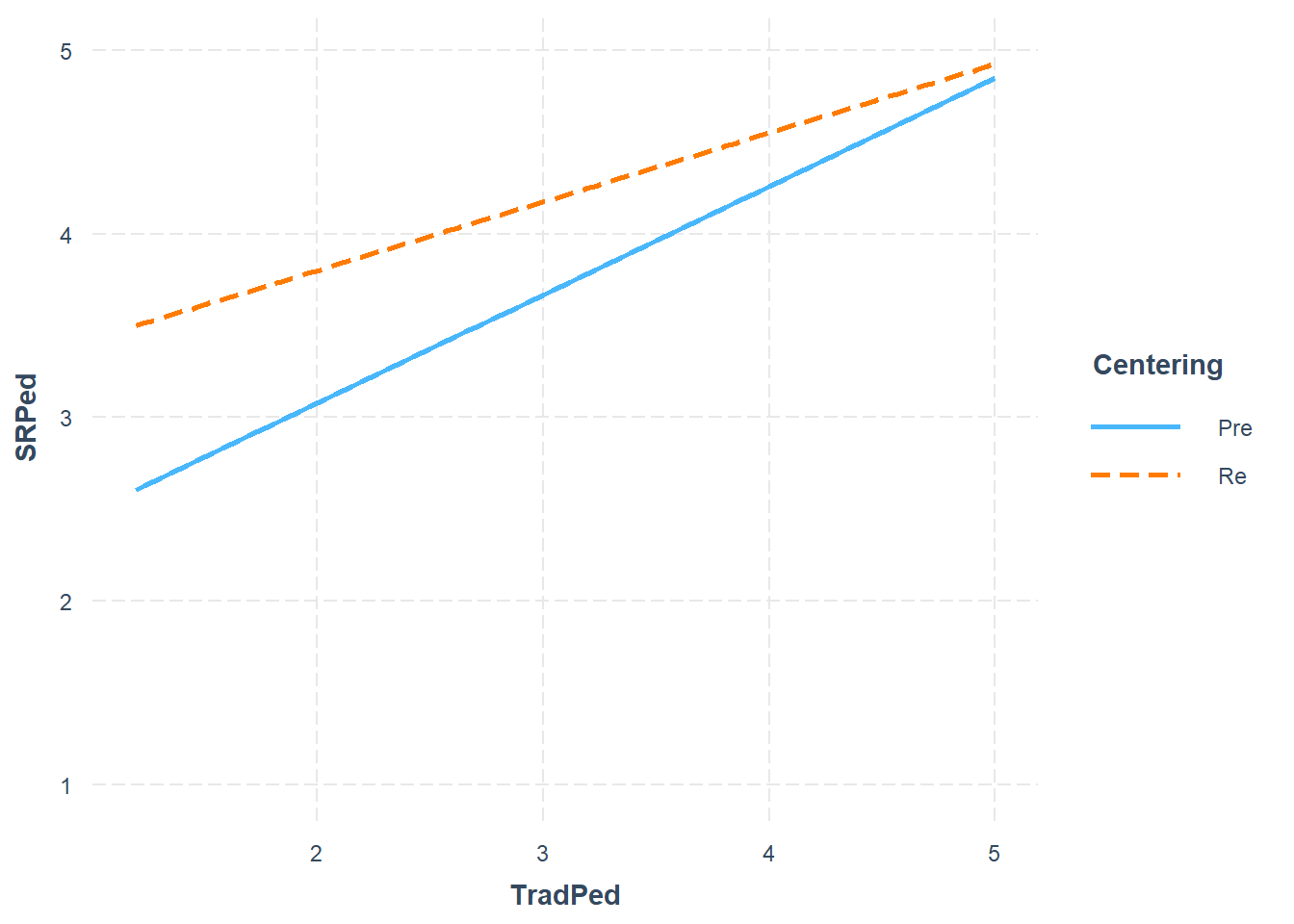
8.11 Homeworked Example 2: A moderation on the b path
For more information about the data used in this homeworked example, please refer to the description and codebook located at the end of the introductory lesson in ReCentering Psych Stats. An .rds file which holds the data is located in the Worked Examples folder at the GitHub site the hosts the OER. The file name is ReC.rds.
The suggested practice problem for this chapter is to conduct a moderated mediation. At least one path (a or b) should be moderated.
Describing they overall model hypothesis, assign each variable to the X, Y, M, and W roles
My analysis will evaluated a moderated mediation. Specifically, I predict that the effect of centering on perceived value to the student will be moderated by the students’ evaluation of socially responsive pedagogy. I further hypothesize that this indirect effect will be moderated by traditional pedagogy and that the moderation will occur on the b path, that is, traditional pedagogy will moderate the relationship between socially responsive pedagogy and perceived value to the student.
- X = Centering, pre/re (0,1)
- W = Traditional Pedagogy (1 to 4 scaling)
- M = Socially Responsive Pedagogy (1 to 4 scaling)
- Y = Value to the student (1 to 4 scaling)
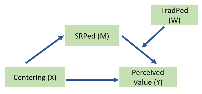
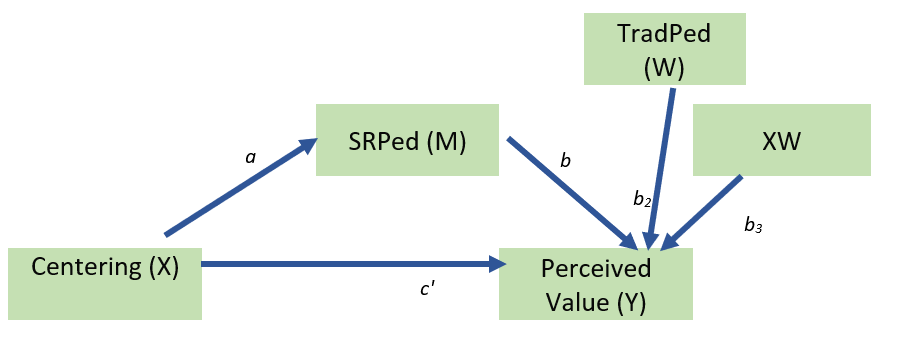
Import the data and format the variables in the model
The approach we are taking to moderated mediation does not allow dependency in the data. Therefore, we will include only those who took the multivariate class (i.e., excluding responses for the ANOVA and psychometrics courses).
I need to score the SRPed, TradPed, and Valued variables
TradPed_vars <- c("ClearResponsibilities", "EffectiveAnswers", "Feedback",
    "ClearOrganization", "ClearPresentation")
raw$TradPed <- sjstats::mean_n(raw[, ..TradPed_vars], 0.75)

Valued_vars <- c("ValObjectives", "IncrUnderstanding", "IncrInterest")
raw$Valued <- sjstats::mean_n(raw[, ..Valued_vars], 0.75)

SRPed_vars <- c("InclusvClassrm", "EquitableEval", "MultPerspectives",
    "DEIintegration")
raw$SRPed <- sjstats::mean_n(raw[, ..SRPed_vars], 0.75)
I will create a babydf.
Let’s check the structure of the variables:
## Classes 'data.table' and 'data.frame':   84 obs. of  4 variables:
##  $ Centering: Factor w/ 2 levels "Pre","Re": 2 2 2 2 2 2 2 2 2 2 ...
##  $ TradPed  : num  3.8 5 4.8 4 4.2 3 5 4.6 4 4.8 ...
##  $ SRPed    : num  4.5 5 5 5 4.75 4.5 5 4.5 5 5 ...
##  $ Valued   : num  4.33 5 4.67 3.33 4 3.67 5 4 4.67 4.67 ...
##  - attr(*, ".internal.selfref")=<externalptr>
In later analyses, it will be important that Centering is a dummy-coded numerical variable:
babydf$CENTERING <- as.numeric(babydf$Centering)
babydf$CENTERING <- (babydf$CENTERING - 1)
str(babydf)
## Classes 'data.table' and 'data.frame': 84 obs. of 5 variables:
## $ Centering: Factor w/ 2 levels "Pre","Re": 2 2 2 2 2 2 2 2 2 2 ...
## $ TradPed : num 3.8 5 4.8 4 4.2 3 5 4.6 4 4.8 ...
## $ SRPed : num 4.5 5 5 5 4.75 4.5 5 4.5 5 5 ...
## $ Valued : num 4.33 5 4.67 3.33 4 3.67 5 4 4.67 4.67 ...
## $ CENTERING: num 1 1 1 1 1 1 1 1 1 1 ...
## - attr(*, ".internal.selfref")=<externalptr>Quick peek at relations between variables:

Using a piecewise approach, run each of the simple models in the grander design
Analysis #1: A simple moderation
We are asking, “Does traditional pedagogy moderate the relationship between socially responsive pedagogy and perceived value to the student?
Y = perceived value to the student X = socially responsive pedagogy W = traditional pedagogy
Let’s specify this simple moderation model with base R’s lm() function.
Mod_b_path <- lm(Valued ~ SRPed * TradPed, data = babydf)
# the base R output if you prefer this view
summary(Mod_b_path)
##
## Call:
## lm(formula = Valued ~ SRPed * TradPed, data = babydf)
##
## Residuals:
## Min 1Q Median 3Q Max
## -1.06146 -0.26683 0.08376 0.19957 0.94852
##
## Coefficients:
## Estimate Std. Error t value Pr(>|t|)
## (Intercept) 1.97179 1.29638 1.521 0.132
## SRPed -0.19009 0.33922 -0.560 0.577
## TradPed 0.35774 0.32949 1.086 0.281
## SRPed:TradPed 0.07962 0.07850 1.014 0.314
##
## Residual standard error: 0.4393 on 77 degrees of freedom
## (3 observations deleted due to missingness)
## Multiple R-squared: 0.6114, Adjusted R-squared: 0.5963
## F-statistic: 40.39 on 3 and 77 DF, p-value: 0.0000000000000008713We’ll use the jtools package so we get that great summ function and interactions for the awesome plot.
Since we are just working to understand our moderation, we can run them with “regular old” ordinary least squares.
# library(jtools) #the summ function creates a terrific regression
# table library(interactions)
library(ggplot2)

jtools::summ(Mod_b_path, digits = 3)| Observations | 81 (3 missing obs. deleted) |
| Dependent variable | Valued |
| Type | OLS linear regression |
| F(3,77) | 40.389 |
| R² | 0.611 |
| Adj. R² | 0.596 |
| Est. | S.E. | t val. | p | |
|---|---|---|---|---|
| (Intercept) | 1.972 | 1.296 | 1.521 | 0.132 |
| SRPed | -0.190 | 0.339 | -0.560 | 0.577 |
| TradPed | 0.358 | 0.329 | 1.086 | 0.281 |
| SRPed:TradPed | 0.080 | 0.078 | 1.014 | 0.314 |
| Standard errors: OLS |
Looking at these results we can see that the predictors account for about 61% of variance in disengagement coping. Only the moderator (W), traditional pedagogy is a significant predictor. Neither the independent variable (Centering, [X])), nor its interaction with Centering (Centering:TradPed, [XW]) are significant.
It’s always helpful to graph the relationship. The interaction_plot() function from the package, interactions can make helpful illustrations. This plot represents the model we specified with each of the variables in their respective roles.
## Warning: 5.02351626747081 is outside the observed range of TradPed Even though this graphs looks as though socially responsive pedagogy leads to higher perceived value (a gentle, positive slope) the non-significant main effect indicates this slope is not statistically significant.
Further, even though it appears that higher ratings of traditional pedagogy are associated with greater perceived value, this main effect was also non-significant.
Consistent with the non-significant interaction effect, there is no evidence of an interaction effect in the figure.
## Warning: 5.02351626747081 is outside the observed range of TradPed## JOHNSON-NEYMAN INTERVAL
##
## The Johnson-Neyman interval could not be found. Is the p value for your
## interaction term below the specified alpha?
##
## SIMPLE SLOPES ANALYSIS
##
## Slope of SRPed when TradPed = 3.599941 (- 1 SD):
##
## Est. S.E. t val. p
## ------ ------ -------- ------
## 0.10 0.13 0.77 0.44
##
## Slope of SRPed when TradPed = 4.311728 (Mean):
##
## Est. S.E. t val. p
## ------ ------ -------- ------
## 0.15 0.12 1.25 0.22
##
## Slope of SRPed when TradPed = 5.023516 (+ 1 SD):
##
## Est. S.E. t val. p
## ------ ------ -------- ------
## 0.21 0.14 1.46 0.15# interactions::sim_slopes(Mod_b_path, pred=TradPed, modx = SRPed)
# #sometimes I like to look at it in reverse -- like in the plotsConsistent with both the non-significant interaction term and the the non-significant main effect of socially responsive pedagogy, there was not statistically significant effect of socially responsive pedagogy on perceived value to the student at the traditional values of the mean (4.31) and \(\pm1SD\) (3.60, 5.02) of the moderator, traditional pedagogy.
Analysis #2: A simple mediation
We are asking, “Does socially responsive pedagogy mediate the relationship between centering and perceived value to the student?”
Y = perceived value X = centering M = socially responsive pedagogy
Note. I switched to using the CENTERING (all caps) variable because it is 0/1, numeric (better for lavaan).
library(lavaan)

medmodel <- "
          Valued ~ b*SRPed + c_p*CENTERING
          SRPed ~a*CENTERING

          #intercepts
          CENTERING ~ CENTERING.mean*1
          Valued ~ Valued.mean*1

          indirect :=  a*b
          direct  := c_p
          total_c  := c_p + (a*b)
          "
set.seed(230925)  #required for reproducible results because lavaan introduces randomness into the calculations
medmodel_fit <- lavaan::sem(medmodel, data = babydf, se = "bootstrap",
    missing = "fiml")
medmodel_Sum <- lavaan::summary(medmodel_fit, standardized = T, rsq = T,
    ci = TRUE)
medmodel_ParEsts <- lavaan::parameterEstimates(medmodel_fit, boot.ci.type = "bca.simple",
    standardized = TRUE)
medmodel_Sum
## lavaan 0.6.17 ended normally after 25 iterations
##
## Estimator ML
## Optimization method NLMINB
## Number of model parameters 9
##
## Number of observations 84
## Number of missing patterns 2
##
## Model Test User Model:
##
## Test statistic 0.000
## Degrees of freedom 0
##
## Parameter Estimates:
##
## Standard errors Bootstrap
## Number of requested bootstrap draws 1000
## Number of successful bootstrap draws 1000
##
## Regressions:
## Estimate Std.Err z-value P(>|z|) ci.lower ci.upper
## Valued ~
## SRPed (b) 0.728 0.124 5.877 0.000 0.455 0.933
## CENTERIN (c_p) 0.004 0.124 0.032 0.974 -0.225 0.257
## SRPed ~
## CENTERIN (a) 0.367 0.114 3.225 0.001 0.148 0.601
## Std.lv Std.all
##
## 0.728 0.608
## 0.004 0.003
##
## 0.367 0.307
##
## Intercepts:
## Estimate Std.Err z-value P(>|z|) ci.lower ci.upper
## CENTERI (CENT) 0.369 0.054 6.872 0.000 0.274 0.476
## .Valued (Vld.) 0.935 0.548 1.707 0.088 0.018 2.136
## .SRPed 4.371 0.086 50.597 0.000 4.187 4.527
## Std.lv Std.all
## 0.369 0.765
## 0.935 1.355
## 4.371 7.580
##
## Variances:
## Estimate Std.Err z-value P(>|z|) ci.lower ci.upper
## .Valued 0.299 0.055 5.453 0.000 0.186 0.408
## .SRPed 0.301 0.058 5.157 0.000 0.196 0.413
## CENTERING 0.233 0.014 16.390 0.000 0.199 0.249
## Std.lv Std.all
## 0.299 0.629
## 0.301 0.906
## 0.233 1.000
##
## R-Square:
## Estimate
## Valued 0.371
## SRPed 0.094
##
## Defined Parameters:
## Estimate Std.Err z-value P(>|z|) ci.lower ci.upper
## indirect 0.267 0.100 2.665 0.008 0.095 0.488
## direct 0.004 0.124 0.032 0.974 -0.225 0.257
## total_c 0.271 0.144 1.886 0.059 -0.014 0.551
## Std.lv Std.all
## 0.267 0.187
## 0.004 0.003
## 0.271 0.190## lhs op rhs label est se z pvalue ci.lower
## 1 Valued ~ SRPed b 0.728 0.124 5.877 0.000 0.464
## 2 Valued ~ CENTERING c_p 0.004 0.124 0.032 0.974 -0.225
## 3 SRPed ~ CENTERING a 0.367 0.114 3.225 0.001 0.131
## 4 CENTERING ~1 CENTERING.mean 0.369 0.054 6.872 0.000 0.262
## 5 Valued ~1 Valued.mean 0.935 0.548 1.707 0.088 -0.040
## 6 Valued ~~ Valued 0.299 0.055 5.453 0.000 0.213
## 7 SRPed ~~ SRPed 0.301 0.058 5.157 0.000 0.205
## 8 CENTERING ~~ CENTERING 0.233 0.014 16.390 0.000 0.199
## 9 SRPed ~1 4.371 0.086 50.597 0.000 4.189
## 10 indirect := a*b indirect 0.267 0.100 2.665 0.008 0.109
## 11 direct := c_p direct 0.004 0.124 0.032 0.974 -0.225
## 12 total_c := c_p+(a*b) total_c 0.271 0.144 1.886 0.059 -0.025
## ci.upper std.lv std.all std.nox
## 1 0.939 0.728 0.608 0.608
## 2 0.250 0.004 0.003 0.003
## 3 0.587 0.367 0.307 0.307
## 4 0.476 0.369 0.765 0.765
## 5 2.084 0.935 1.355 1.355
## 6 0.454 0.299 0.629 0.629
## 7 0.424 0.301 0.906 0.906
## 8 0.249 0.233 1.000 1.000
## 9 4.528 4.371 7.580 7.580
## 10 0.528 0.267 0.187 0.187
## 11 0.250 0.004 0.003 0.003
## 12 0.546 0.271 0.190 0.190# only worked when I used the library to turn on all these pkgs
library(lavaan)
library(dplyr)
library(ggplot2)
library(tidySEM)
tidySEM::graph_sem(model = medmodel_fit)
We can use the tidySEM::get_layout function to understand how our model is being mapped.
##      [,1]        [,2]
## [1,] "CENTERING" NA
## [2,] "SRPed"     "Valued"
## attr(,"class")
## [1] "layout_matrix" "matrix"        "array"
We can write code to remap them
##      [,1]        [,2]    [,3]
## [1,] ""          "SRPed" ""
## [2,] "CENTERING" ""      "Valued"
## attr(,"class")
## [1] "layout_matrix" "matrix"        "array"
We can update the tidySEM::graph_sem function with our new model to produce something that will better convey our analyses and its results.
tidySEM::graph_sem(medmodel_fit, layout = medmap, rect_width = 1.25, rect_height = 1.25,
    spacing_x = 2, spacing_y = 3, text_size = 4.5)
### Specify and run the entire lavaan model {-}
set.seed(230925)
ModMedOnB <- "
    #equations
    SRPed ~ a*CENTERING
    Valued ~ cp*CENTERING + b1*SRPed + b2*TradPed + b3*SRPed:TradPed

    #intercepts
    SRPed ~ SRPed.mean*1
    Valued ~ Valued.mean*1

    #means, variances of W for simple slopes
    TradPed ~ TradPed.mean*1
    TradPed ~~ TradPed.var*TradPed

    #index of moderated mediation, there will be an a and b path in the product
    #if the a and/or b path is moderated, select the label that represents the moderation

    imm := a*b3

    #Note that we first create the indirect product, then add to it the product of the imm and the W level
    indirect.SDbelow := a*b1 + imm*(TradPed.mean - sqrt(TradPed.var))
    indirect.mean := a*b1 + imm*(TradPed.mean)
    indirect.SDabove := a*b1 + imm*(TradPed.mean + sqrt(TradPed.var))

 "
set.seed(230925)  #required for reproducible results because lavaan introduces randomness into the calculations
ModMedOnB_fit <- lavaan::sem(ModMedOnB, data = babydf, se = "bootstrap",
    missing = "fiml", bootstrap = 1000)
## Warning in lav_partable_vnames(FLAT, "ov.x", warn = TRUE): lavaan WARNING:
## model syntax contains variance/covariance/intercept formulas
## involving (an) exogenous variable(s): [TradPed]; These variables
## will now be treated as random introducing additional free
## parameters. If you wish to treat those variables as fixed, remove
## these formulas from the model syntax. Otherwise, consider adding
## the fixed.x = FALSE option.ModMedOnBsum <- lavaan::summary(ModMedOnB_fit, standardized = TRUE, rsq = T,
ci = TRUE)
ModMedOnBParamEsts <- lavaan::parameterEstimates(ModMedOnB_fit, boot.ci.type = "bca.simple",
standardized = TRUE)
ModMedOnBsum## lavaan 0.6.17 ended normally after 29 iterations
##
## Estimator ML
## Optimization method NLMINB
## Number of model parameters 13
##
## Number of observations 84
## Number of missing patterns 3
##
## Model Test User Model:
##
## Test statistic 390.225
## Degrees of freedom 5
## P-value (Chi-square) 0.000
##
## Parameter Estimates:
##
## Standard errors Bootstrap
## Number of requested bootstrap draws 1000
## Number of successful bootstrap draws 1000
##
## Regressions:
## Estimate Std.Err z-value P(>|z|) ci.lower ci.upper
## SRPed ~
## CENTERING (a) 0.352 0.114 3.077 0.002 0.133 0.590
## Valued ~
## CENTERING (cp) 0.019 0.108 0.174 0.862 -0.195 0.225
## SRPed (b1) 0.060 0.528 0.114 0.909 -1.726 0.436
## TradPed (b2) 0.633 0.497 1.274 0.203 -0.894 0.977
## SRPd:TrdP (b3) 0.014 0.113 0.126 0.900 -0.032 0.396
## Std.lv Std.all
##
## 0.352 0.296
##
## 0.019 0.014
## 0.060 0.055
## 0.633 0.723
## 0.014 0.110
##
## Intercepts:
## Estimate Std.Err z-value P(>|z|) ci.lower ci.upper
## .SRPed (SRP.) 4.382 0.087 50.609 0.000 4.196 4.537
## .Valued (Vld.) 0.939 2.160 0.435 0.664 -0.148 8.017
## TradPed (TrP.) 4.296 0.076 56.560 0.000 4.142 4.434
## SRPd:TP 19.741 0.524 37.679 0.000 18.697 20.707
## Std.lv Std.all
## 4.382 7.627
## 0.939 1.497
## 4.296 5.993
## 19.741 4.104
##
## Variances:
## Estimate Std.Err z-value P(>|z|) ci.lower ci.upper
## TradPed (TrP.) 0.514 0.140 3.681 0.000 0.272 0.803
## .SRPed 0.301 0.059 5.110 0.000 0.195 0.416
## .Valued 0.181 0.029 6.327 0.000 0.111 0.223
## SRPd:TP 23.133 4.269 5.419 0.000 15.303 32.150
## Std.lv Std.all
## 0.514 1.000
## 0.301 0.912
## 0.181 0.461
## 23.133 1.000
##
## R-Square:
## Estimate
## SRPed 0.088
## Valued 0.539
##
## Defined Parameters:
## Estimate Std.Err z-value P(>|z|) ci.lower ci.upper
## imm 0.005 0.040 0.125 0.901 -0.012 0.145
## indirect.SDblw 0.039 0.066 0.593 0.553 -0.122 0.151
## indirect.mean 0.043 0.055 0.784 0.433 -0.074 0.156
## indirect.SDabv 0.046 0.057 0.809 0.418 -0.065 0.165
## Std.lv Std.all
## 0.005 0.032
## 0.039 0.178
## 0.043 0.210
## 0.046 0.243## lhs op rhs
## 1 SRPed ~ CENTERING
## 2 Valued ~ CENTERING
## 3 Valued ~ SRPed
## 4 Valued ~ TradPed
## 5 Valued ~ SRPed:TradPed
## 6 SRPed ~1
## 7 Valued ~1
## 8 TradPed ~1
## 9 TradPed ~~ TradPed
## 10 SRPed ~~ SRPed
## 11 Valued ~~ Valued
## 12 SRPed:TradPed ~~ SRPed:TradPed
## 13 CENTERING ~~ CENTERING
## 14 SRPed:TradPed ~1
## 15 CENTERING ~1
## 16 imm := a*b3
## 17 indirect.SDbelow := a*b1+imm*(TradPed.mean-sqrt(TradPed.var))
## 18 indirect.mean := a*b1+imm*(TradPed.mean)
## 19 indirect.SDabove := a*b1+imm*(TradPed.mean+sqrt(TradPed.var))
## label est se z pvalue ci.lower ci.upper std.lv std.all
## 1 a 0.352 0.114 3.077 0.002 0.117 0.573 0.352 0.296
## 2 cp 0.019 0.108 0.174 0.862 -0.201 0.223 0.019 0.014
## 3 b1 0.060 0.528 0.114 0.909 -1.264 0.564 0.060 0.055
## 4 b2 0.633 0.497 1.274 0.203 -0.889 0.982 0.633 0.723
## 5 b3 0.014 0.113 0.126 0.900 -0.032 0.396 0.014 0.110
## 6 SRPed.mean 4.382 0.087 50.609 0.000 4.191 4.537 4.382 7.627
## 7 Valued.mean 0.939 2.160 0.435 0.664 -0.117 8.165 0.939 1.497
## 8 TradPed.mean 4.296 0.076 56.560 0.000 4.137 4.431 4.296 5.993
## 9 TradPed.var 0.514 0.140 3.681 0.000 0.275 0.811 0.514 1.000
## 10 0.301 0.059 5.110 0.000 0.205 0.430 0.301 0.912
## 11 0.181 0.029 6.327 0.000 0.141 0.281 0.181 0.461
## 12 23.133 4.269 5.419 0.000 15.792 33.016 23.133 1.000
## 13 0.233 0.000 NA NA 0.233 0.233 0.233 1.000
## 14 19.741 0.524 37.679 0.000 18.724 20.761 19.741 4.104
## 15 0.369 0.000 NA NA 0.369 0.369 0.369 0.765
## 16 imm 0.005 0.040 0.125 0.901 -0.011 0.147 0.005 0.032
## 17 indirect.SDbelow 0.039 0.066 0.593 0.553 -0.056 0.197 0.039 0.178
## 18 indirect.mean 0.043 0.055 0.784 0.433 -0.046 0.179 0.043 0.210
## 19 indirect.SDabove 0.046 0.057 0.809 0.418 -0.063 0.167 0.046 0.243
## std.nox
## 1 0.613
## 2 0.030
## 3 0.055
## 4 0.487
## 5 0.110
## 6 7.627
## 7 1.497
## 8 5.993
## 9 1.000
## 10 0.912
## 11 0.461
## 12 1.000
## 13 0.233
## 14 4.104
## 15 0.369
## 16 0.067
## 17 0.369
## 18 0.436
## 19 0.503Use tidySEM to create a figure
# only worked when I used the library to turn on all these pkgs
library(lavaan)
library(dplyr)
library(ggplot2)
library(tidySEM)
tidySEM::graph_sem(model = ModMedOnB_fit)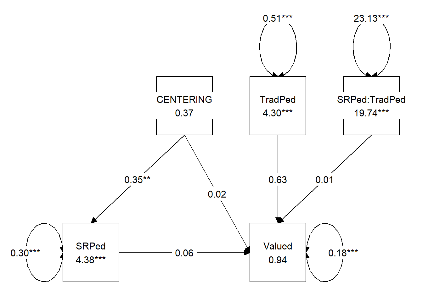
We can use the tidySEM::get_layout function to understand how our model is being mapped.
##      [,1]    [,2]        [,3]      [,4]
## [1,] NA      "CENTERING" "TradPed" "SRPed:TradPed"
## [2,] "SRPed" NA          "Valued"  NA
## attr(,"class")
## [1] "layout_matrix" "matrix"        "array"
We can write code to remap them
comb_map <- tidySEM::get_layout("", "SRPed", "TradPed", "SRPed:TradPed",
    "CENTERING", "", "Valued", "", rows = 2)
comb_map
## [,1] [,2] [,3] [,4]
## [1,] "" "SRPed" "TradPed" "SRPed:TradPed"
## [2,] "CENTERING" "" "Valued" ""
## attr(,"class")
## [1] "layout_matrix" "matrix" "array"We can update the tidySEM::graph_sem function with our new model to produce something that will better convey our analyses and its results.
tidySEM::graph_sem(ModMedOnB_fit, layout = comb_map, rect_width = 1.25,
    rect_height = 1.25, spacing_x = 2, spacing_y = 3, text_size = 3.5)
Create a table that includes regression output for the M and Y variables and the moderated effects
Exporting the results to a .csv file will help us create a journal-ready table, outside of the R environment.
Table 1
| Analysis of Moderated Mediation for Centering, Socially Responsive Pedagogy, Traditional Pedagogy, and Perceived Value to the Student |
|---|
| Predictor | \(B\) | \(SE_{B}\) | \(p\) | \(R^2\) |
|---|
| Socially Responsive Pedagogy(M) | .09 | |||
|---|---|---|---|---|
| Constant | 4.382 | 0.087 | <0.001 | |
| Centering (\(a\)) | 0.352 | 0.114 | 0.002 |
| Perceived Value (DV) | .54 | |||
|---|---|---|---|---|
| Constant | 0.939 | 2.160 | 0.664 | |
| Centering (\(c'\)) | 0.019 | 0.108 | 0.862 | |
| SRPed (\(b_1\)) | 0.060 | 0.528 | 0.909 | |
| TradPed (\(b_2\)) | 0.633 | 0.497 | 0.203 | |
| SRPed:TradPed (\(b_3\)) | 0.014 | 0.113 | 0.900 |
| Summary of Effects | \(B\) | \(SE_{B}\) | \(p\) | 95% CI |
|---|---|---|---|---|
| IMM | 0.005 | 0.040 | 0.901 | -0.011, 0.147 |
| Indirect (\(-1SD\)) | 0.039 | 0.066 | 0.553 | -0.056, 0.197 |
| Indirect (\(M\)) | 0.043 | 0.055 | 0.433 | -0.046, 0.179 |
| Indirect (\(+1SD\)) | 0.046 | 0.057 | 0.418 | -0.063 0.167 |
| Note. SRPed = socially responsive pedagogy; TradPed = traditional pedagogy. The significance of the indirect effects was calculated with bootstrapped, bias-corrected, confidence intervals (.95). |
APA Style Write-up
Method/Analytic Strategy
Data were analyzed with a maximum likelihood approach the package, lavaan (v. 0.6-16). We specified a moderated mediation model predicting perceived value to the student from centering stage, mediated by socially responsive pedagogy. We further predicted that the relationship between socially responsive pedagogy to perceived value (i.e., the b path) would be moderated by traditional pedagogy.
Results
Preliminary Analyses
- Missing data anlaysis and managing missing data
- Bivariate correlations, means, SDs
- Distributional characteristics, assumptions, etc.
- Address limitations and concerns
Primary Analyses Our analysis evaluated a moderation mediation model perceived value to the student (Y/Valued) from centering stage (X/Centering) mediated by socially responsive pedagogy (M/SRPed). Traditional pedagogy (W/TradPed) was our moderating variable. We specified a moderation of path b (M/SRPed to Y/Valued). Data were analyzed with maximum likelihood estimation in the R package lavaan (v. 0.6-16); the significance of effects were tested with 1000 bootstrap confidence intervals. Results of the full model are presented in Table 1 and illustrated in Figure 1. The formula for the mediator and dependent variable are expressed below.
\[\hat{M} = 4.382 + 0.352X\] \[\hat{Y} = 0.939 + (0.019)X + (0.060)M + (0.633)W + 0.014MW \]
Although the model accounted for 9% of variance in socially responsive pedagogy (mediator) and 54% of variance in the perceived value to the student (dependent variable), results suggested non significant main, interaction, and mediated effects. Correspondingly, the index of moderated mediation was not significant \((B = 0.005, p = 0.901, 95CI(-0.011, 0.147)\), suggesting that the indirect effects were not conditional on the values of the moderator. Figure 1 illustrates the conditional effects (all non-significant) of socially responsive pedagogy (M) on perceived value to the student (Y) among across the \(M \pm 1SD\) of the moderator, traditional pedagogy. Complete results are found in Table 1.
## Warning: 5.02351626747081 is outside the observed range of TradPed