Chapter 13 Preliminary (OLS style) Exploration of Longitudinal Growth
This lesson is an introduction to longitudinal modeling when time is a factor. In this lecture we explore the longitudinal data using OLS tools. Doing so provides the proper screening/vetting of the data to ensure that it is appropriate for multilevel analysis. Simultaneously, it provides an orientation to the types of questions that MLM will address.
13.2 Change-Over-Time Analytics
There are a host of ways to investigate change over time: longitudinal SEM, latent growth curve modeling, latent mixture models, and so forth. We are focused on the subset of this approach that has so many names: individual growth curve models, random coefficient models, multilevel models, linear mixed effects models, hierachical linear models.
Before we start down the longitudinal/repeated measures path, a note to say that this class of statistics was born out of a need to deal with dependency in the data and it applies to both cross-sectional and longitudinal/repeated measures models.
- Remember ANOVA? (Excepting repeated measure or mixed design ANOVA) One of the statistical assumptions was that the data had to be independent. That is, you could not have family members, co-workers, etc., in the dataset because their data would likely be correlated.
- In the context of these related circumstances (students in a classroom, supervisees of a manager) researchers were confused about how to handle the data. Should they aggregate the dependent data (effectively reduce the sample size by taking the mean of all those in a dependent cluster and using it with the non-dependent data)? Should they keep it disaggregated (effectively repeating/copying the non-dependent data for each member of the cluster)? Each approach was fraught with difficulty.
Random coefficient regression models (RCR or RCM) are an effective alternative to ordinary least squares (OLS) to account for dependencies within the data. The math and approach toward longitudinal modeling is largely the same as when we manage dependencies cross-sectional studies (e.g., members of a team, supervisors reporting to a leader/manager). A more thorough review of aggregation and disaggregation can be found in the ReCentering Psych Stats chapter devoted to cross-sectional data.
 This class of analysis allows us to address questions about:
- Within-individual change: How does each person change over time?
- These are descriptive questions: Is change linear? nonlinear? consistent? fluctuating?
- level-1 concerns within-individual change over time
- individual growth trajectory – the way outcome values rise and fall over time
- Goal is to describe the shape of each person’s growth trajectory
- Interindividual differences in change: What predicts differences among people in their changes?
- A relational question: What is the association between predictors and patterns of change? Are these relations moderated?
- level-2 concerns interindividual differences in change
- Do different people manifest different patterns of within-individual change? What predicts these differences?
- Goal is to detect heterogeneity in change across individuals and to determine the relationship between predictors and the shape of each person’s individual growth trajectory.
Together, we map the research questions onto a linked pair of statistical models known as the multilevel model for change:
- a level-1 (L1) model, describing within-individual change over time; and
- a level-2 (L2) model, relating predictors to any interindividual differences in change
Asking these questions requires three criteria of the research design/data:
- Multiple waves of data
- Contrast with a developmental psychologist analyzing cross-sectional data composed of children of differing ages. In spite of compelling (and totally fine) research designs, the cross-sectional nature of the design can not rule out plausible rival hypotheses.
- Contrast with two waves of data. Singer and Willett (2003) state that these data, “are only marginally better” (p. 10). Two-wave researchers argued in favor of their increment (i.e, the simple difference between scores assessed on the two measurement occasions). Even if the increment is large, Singer and Willett (2003) argue that the increment cannot describe the process of change because it cannot describe the shape (the focus of the level-1 question). Singer and Willett further argue that two-wave studies cannot describe individual change trajectories because they confound true change with measurement error.
- How many waves? Within cost and logistical constraints, “more waves are always better.” More allows more complex modeling. The statistical rule is that you need one-more-wave than the shape you wish to model. For example, you need 2 waves for a straight line (linear model), 3 waves for a quadratic (1 hump) model, 4 waves for a cubic (2 curves) model, and so forth.
- A substantively meaningful metric for time
- “Time is the fundamental predictor in every study of change; it must be measured reliably and validly in a sensible metric” (p. 10).
- What is sensible? ages, grades, months-since-intake, miles, etc. The choice of metric affects related decisions including number and spacing of waves.
- Consider the cadence you expect in the outcome. Weeks or number of sessions is sensible for psychotherapy studies. Grade or age is sensible for education. Parental or child age might make sense for parenting.
- “The temporal variable can change only monotonically” (p. 12), that is, it cannot reverse diretions. This means you can have height as a temporal variable, but not weight.
- There is NOTHING SACRED about evenly spaced variables. In fact, if you expect rapid nonlinear change during some periods, you should collect mored data at those times. If you expect little movement, you can maybe space them urther apart.
- Time-structured schedules assess all participants on an identical schedule (cb equally or unequally spaced). Time-unstructured schedules allow data collection schedules to vary across individuals. Multi-level modeling can accomodate both.
- No requirement for balance. That is, each person can have a different number of waves. While non-random attrition can be problematic for drawing inferences, individual growth modeling does not require balanced data.
- An outcome that changes systematically
- The content of measurement is a substantive, not statistical decision. However…
- How the construct is measured is a statistical decision and “not all variables are equally suited” (p. 13). Individual growth models are designed for continuous outcomes whose values change systematically over time.
- Continuous outcomes are those that support “all the usual manipulations of arithmetic” (p. 13). That is, you can take differences between pairs of scores, add, subtract, multiply, divide. Most psychometrically credible instruments will work. BUT!
- the “metric, validity, and precision” of the outcome must be preserved across time. That is, the outcome scores must be “equatable over time”. That is, a given value of the outcome on any occasion must represent the same “amount” of the outcome on every occasion. Outcome equatability is supported (in part) by using the identical instrument each time.
- Standardization in the longitudinal context is hotly debated and not a simple solution for equating shifty metrics. Why? the SD units likely have different size/meaning at different intervals. Transforming the M to 0.0 and the SD to 1.0 masks the variance differences that may exist. The raw metric preserves the variance and avoids all the issues.
- Outcomes should be equally valid across all measurement occasions. For example, a multiplication test may be a valid measure of mathematical skill among young children, but a measure of memory among teenagers.
- Although precision need not be identical at every occasion, the goal is to minimize errors introduced by instrument administration. Look for reliabilities of .8 and above.
“Structuring up” a longitudinal data set and engaging in preliminary data anlaysis is a great way to further understand this approach to statistical modeling. So, let’s transition to our research vignette.
13.4 Research Vignette
Our research vignette (Lefevor et al., 2017) examines the intersection of religious and sexual identities of clients in therapy. With 12,825 participants from the Center for Collegiate Mental Health 2012-2014 data set, the project is an example of working with big data. Because the data is available to members only (and behind a paywall), I simulated the data. In the simulation, categorical variables (e.g., sexual identity, session number, religious identity) were rendered as continuous variables and in the simulation, I needed to transform them back into categorical ones. Inevitably, this will have introduced a great deal of error. Thus, we can expect that the results from the simulated data will be different from those obtained by the authors.
The Method section of the article provides detailed information about the inclusion criteria ofr the study and the coding of the variables. This included data about the religious and sexual identities as well as a minimum of three separate scores on the Counseling Center Assessment of Psychologial Sympsoms (CCAPS, Locke et al., 2012) measure. For the final dataset, clients attended an average of 10.58 sessions (SD = 7.65) and had an average of 5.36 CCAPS administrations (SD = 4.04). This means that in the original dataset, each client was represented by a varying number of observations (likely ranging from 3 [the minimum required for inclusion] and, perhaps as many as 17 [adding +3SDs to the mean CCAPS administrations]). In simulating the data, I specified five observations for each of the 12,825 clients.
Let’s take a look at the variables in the study
Anxiety and Depression: The anxiety and depression ratings were taken from the CCAPS measure (Locke et al., 2012) that assesses psychological distress across seven domains. Clients rate themselves over the past two weeks on a 5-point Likert-type scale ranging from 0 (not at all like me) to 4 (extremely like me). Higher scores indicate more distress. The dataset comes from multiple institutions with different procedures around assessment CCAPS there is not a 1:1 correspondence with session number and CCAPS assessment.
Sexual Identity: Sexual identity was dichotomized into heterosexual (-1, 85.5%) and LGBQQ (1, 14.5%).
Relious Identity: Religious identity was coded into three categories including dominant religious (DR; Christian, Catholic), nondominant religious (NDR; Muslim, Hindu, Buddhist, Jewish), and nondominant unaffiliated (NDU; agnostic, atheist, no preference). The three categories were contrast coded with an orthogonal contrast-coding scheme with two variables. The first variable compared DR(coded as 2) to NDU and NDR (coded as -1); the second variable compared the two nondominant groups (NDU = -1, DR = 0, NDR = 1).
13.4.1 Simulating the data from the journal article
#calculations for the simulation
#SD estimated by multiplying SE by square root of N
.02 *sqrt(12825)
#SD for anxiety in empty model
.02*sqrt(12825)

#Range (+/- 3SD) for anxiety in Mod5
2.03 - 3*(.02 *sqrt(12825))
2.03 + 3*(.02 *sqrt(12825))

#Range (+/- 3SD) for session in Mod5
-.22 - 3*(.01 *sqrt(12825))
-.22 + 3*(.01 *sqrt(12825))

#Range (+/- 3SD) for sexual identity in Mod5
.13 - 3*(.02 *sqrt(12825))
.13 + 3*(.02 *sqrt(12825))

#Range (+/- 3SD) for Religious 1 in Mod4
-.03 - 3*(.01 *sqrt(12825))
-.03 + 3*(.01 *sqrt(12825))

#Range (+/- 3SD) for Religious 1 in Mod4
.01 - 3*(.01 *sqrt(12825))
.01 + 3*(.01 *sqrt(12825))set.seed(200513)
n_client = 12825
n_session = 5
b0 = 2.03 #intercept for anxiety
b1 = -0.22 #b weight for L1 session
b2 = 0.13 #b weight for L2 sexual identity
b3 = -0.03 #b weight for L2 Rel1 (D-R vs ND-R & ND-U)
b4 = 0.01 #b weight for the L2 Rel2 (ND-R vs ND-U)
# the values used below are the +/- 3SD they produce continuous
# variables which later need to be transformed to categorical ones;
# admittedly this introduces a great deal of error/noise into the
# simulation the article didn't include a correlation matrix or M/SDs
# so this was a clunky process
(Session = runif(n_client * n_session, -3.61, 3.18)) #calc L1 Session, values are the +/3 3SD
(SexualIdentity = runif(n_client * Session, -6.66, 6.92)) #calc L2 Sexual Identity, values are the +/3 3SD
(Religion1 = runif(n_client * Session, -3.43, 3.37)) #calc L2 Religion1, values are the +/3 3SD
(Religion2 = rep(runif(n_session, -3.38, 3.41), each = n_session)) #calc L2 Religion2, values are the +/3 3SD
mu = 1.76 #intercept of empty model
sds = 2.264 #this is the SD of the DV
sd = 1 #this is the observation-level random effect variance that we set at 1
# ( church = rep(LETTERS[1:n_church], each = n_mbrs) ) #this worked
# in the prior
(client = rep(LETTERS[1:n_client], each = n_session))
# ( session = numbers[1:(n_client*n_session)] )
(clienteff = rnorm(n_client, 0, sds))
(clienteff = rep(clienteff, each = n_session))
(sessioneff = rnorm(n_client * n_session, 0, sd))
(Anxiety = b0 + b1 * Session + b2 * SexualIdentity + b3 * Religion1 + b4 *
Religion2 + clienteff + sessioneff)
(dat = data.frame(client, clienteff, sessioneff, Session, SexualIdentity,
Religion1, Religion2, Anxiety))
library(dplyr)##
## Attaching package: 'dplyr'## The following objects are masked from 'package:stats':
##
## filter, lag## The following objects are masked from 'package:base':
##
## intersect, setdiff, setequal, uniondat <- dat %>%
mutate(ID = row_number())
# moving the ID number to the first column; requires
dat <- dat %>%
select(ID, everything())
Lefevor2017 <- dat %>%
select(ID, client, Session, SexualIdentity, Religion1, Religion2, Anxiety)
Lefevor2017$ClientID <- rep(c(1:12825), each = 5)
# rounded Sexual Identity into dichotomous variable 85% were
# heterosexual,
library(robumeta)
# The following variables should be L2, but were simulated as if they
# were L1
Lefevor2017$Rel1 <- as.numeric(group.mean(Lefevor2017$Religion1, Lefevor2017$ClientID)) #aggregated at group mean
Lefevor2017$Rel2 <- as.numeric(group.mean(Lefevor2017$Religion2, Lefevor2017$ClientID)) #aggregated at group mean
Lefevor2017$SxID <- as.numeric(group.mean(Lefevor2017$SexualIdentity, Lefevor2017$ClientID)) #aggregated at group mean
# Rel2 has contrast codes for dominant religion (DR, 0), nondominant
# religious (NDR, 1) and nondominant unspecified (NDU, -1) Strategy
# is to figure out the raw score associated with the percentile rank
# of -1 and 0, to set the breakpoints for the coding NDU coded as -1
# 19.2+13.5+9.6 NDU has bottom 42.3 percent
# DR coded as 0, so quantile cut will be 42.3 + 52.7 = 95th 33.4 +
# 19.3 52.7% of sample (according to article) was DR must look up
# percentile ranks for 5% and 57.5%
# NDR 2.3+1+1+.7 NDR has 5% of sample 42.3+52.7
# quantile(Lefevor2017$Religion2, probs = c(.423, .95)) effects
# coding the second Religion variable so that NDU = -1, DR = 0, NDR =
# 1
Lefevor2017$Rel2L2 <- ifelse(Lefevor2017$Religion2 <= -3.0877087, -1, ifelse(Lefevor2017$Religion2 >=
-3.0877087 & Lefevor2017$Religion2 <= 0.9299491, 0, 1))
# checking work Rel2L2_table <- table(Lefevor2017$Rel2L2)
# prop.table(Rel2L2_table) Lefevor2017 %>% count(Rel2L2)
# creating the first religion variable where DR is 2 and NDR and NDU
# are both -1
Lefevor2017$Rel1L2 <- plyr::mapvalues(Lefevor2017$Rel2L2, from = c(-1,
0, 1), to = c(-1, 2, -1))
Lefevor2017$DRel0 <- plyr::mapvalues(Lefevor2017$Rel2L2, from = c(-1, 0,
1), to = c(1, 0, 1))
# checking to make sure that 52.7% are coded 2 (DR) Rel1L2_table <-
# table(Lefevor2017$Rel1L2) prop.table(Rel1L2_table)
# heterosexual is -1 LGBTQIA+ is 1 quantile(Lefevor2017$SxID, probs =
# c(.85))
Lefevor2017$SexID <- ifelse(Lefevor2017$SxID <= 1.203468, -1, 1)
Lefevor2017$Het0 <- plyr::mapvalues(Lefevor2017$SexID, from = c(-1, 1),
to = c(0, 1))
# SexID_table <- table(Lefevor2017$SexID) prop.table(SexID_table)
# creating a variable representing the session number for each
# client, in the article up to 20 sessions were allowed.
# install.packages('scales')
library(scales)
# Right from the beginning I centered this so that 0 would represent
# intake
Lefevor2017$Session0 <- as.integer(scales::rescale(Lefevor2017$Session,
to = c(0, 19)))
# creating session waves (1 thru 5) by rank ordering within each
# person's variable the continuous variable Session that was created
# in the original simulation
library(dplyr)
Lefevor2017 <- Lefevor2017 %>%
dplyr::group_by(ClientID) %>%
mutate(Index = rank(Session))
# selecting the simulated variables
Lefevor2017_sim <- Lefevor2017 %>%
select(ClientID, Index, Session0, Anxiety, DRel0, Het0)
# In the transition from long-to-wide, it seems like you can only do
# one L1 variable at a time When there are multiple L1 and L2 vars,
# put all L2 vars on left of tilde The wave/index function should
# come next; this should be finite (like integers of 1,2,3,4) with a
# maximum Put the name of the SINGLE L1 variable in the concatonated
# list
library(data.table)##
## Attaching package: 'data.table'## The following objects are masked from 'package:dplyr':
##
## between, first, lastLfvrWp1 <- reshape2::dcast(Lefevor2017_sim, ClientID + DRel0 + Het0 ~ Index,
value.var = c("Index"))
# rename the anxiety variable
LfvrWp1 <- rename(LfvrWp1, Index1 = "1", Index2 = "2", Index3 = "3", Index4 = "4",
Index5 = "5")
LfvrWp2 <- reshape2::dcast(Lefevor2017_sim, ClientID ~ Index, value.var = c("Anxiety"))
# rename the anxiety variable
LfvrWp2 <- rename(LfvrWp2, Anx1 = "1", Anx2 = "2", Anx3 = "3", Anx4 = "4",
Anx5 = "5")
# For remaining L1 variable, do them one at a time -- key them from
# the person-level ID and the wave/index.
LfvrWp3 <- reshape2::dcast(Lefevor2017_sim, ClientID ~ Index, value.var = c("Session0"))
LfvrWp3 <- rename(LfvrWp3, Sess1 = "1", Sess2 = "2", Sess3 = "3", Sess4 = "4",
Sess5 = "5")
# Next, join the dataframes by the person-level ID Only two can be
# joined at a time
LfvrWide <- dplyr::full_join(LfvrWp1, LfvrWp2, by = c("ClientID"))
LfvrWide <- dplyr::full_join(LfvrWide, LfvrWp3, by = c("ClientID"))To increase the portability of the OER, this chapter uses simulated data. Here is script for exporting/downloading the data as a .csv file to your local computer and then importing/uploading it again. I find that saving the .csv file (data) in the same place as the .rmd file(s) is essential for R to connect the two.
Because this simulation can take a few minutes, you may wish to do this, even as you work through this chapter, so that resimulations take less time and comuting resources.
13.5 Longitudinal Exploration
13.5.1 The Structure of the Data File as the First Step in Understanding Longitudinal Modeling
We are accustomed to viewing data in its wide format. The wide format is also technically termed the person-level data set or the multivariate format of data. It is characterized by the following:
- Each person has one record and multiple variables contain the data from each measurement occasion; a 16-person set has 16 records while a 20,000 person set has 20,000 records.
- As you collect additional waves, a person-level file gains new variables (not new cases).
- In the context of longitudinal modeling, data in this form allows us to visually examing an empirical growth record (the temporally sequenced outcomes).
- This wide file arrays each person’s empirical growth record horizontally
There are disadvantages to the wide format:
- The summaries are uninformative.
- It omits an explicit time variable.
- It is inefficient/useless when the number and spacing of waves varies
- It cannot handle the presence of time-varying predictors.
##
## Attaching package: 'psych'
## The following objects are masked from 'package:scales':
##
## alpha, rescale## vars n mean sd median trimmed mad min max
## ClientID 1 12825 6413.00 3702.40 6413.00 6413.00 4753.22 1.00 12825.00
## DRel0 2 12825 0.60 0.49 1.00 0.62 0.00 0.00 1.00
## Het0 3 12825 0.28 0.45 0.00 0.22 0.00 0.00 1.00
## Index1 4 12825 1.00 0.00 1.00 1.00 0.00 1.00 1.00
## Index2 5 12825 2.00 0.00 2.00 2.00 0.00 2.00 2.00
## Index3 6 12825 3.00 0.00 3.00 3.00 0.00 3.00 3.00
## Index4 7 12825 4.00 0.00 4.00 4.00 0.00 4.00 4.00
## Index5 8 12825 5.00 0.00 5.00 5.00 0.00 5.00 5.00
## Anx1 9 12825 2.58 2.54 2.56 2.58 2.52 -7.88 11.88
## Anx2 10 12825 2.32 2.55 2.31 2.33 2.56 -8.13 12.31
## Anx3 11 12825 2.08 2.56 2.06 2.08 2.57 -7.36 12.87
## Anx4 12 12825 1.82 2.52 1.82 1.83 2.52 -7.29 10.72
## Anx5 13 12825 1.58 2.52 1.56 1.58 2.55 -7.58 11.23
## Sess1 14 12825 2.66 2.64 2.00 2.27 2.96 0.00 16.00
## Sess2 15 12825 5.83 3.37 5.00 5.64 2.96 0.00 17.00
## Sess3 16 12825 8.99 3.58 9.00 8.98 4.45 0.00 18.00
## Sess4 17 12825 12.15 3.38 12.00 12.33 4.45 0.00 18.00
## Sess5 18 12825 15.31 2.68 16.00 15.72 2.96 2.00 19.00
## range skew kurtosis se
## ClientID 12824.00 0.00 -1.20 32.69
## DRel0 1.00 -0.41 -1.83 0.00
## Het0 1.00 0.99 -1.02 0.00
## Index1 0.00 NaN NaN 0.00
## Index2 0.00 NaN NaN 0.00
## Index3 0.00 NaN NaN 0.00
## Index4 0.00 NaN NaN 0.00
## Index5 0.00 NaN NaN 0.00
## Anx1 19.76 0.03 0.06 0.02
## Anx2 20.44 -0.02 -0.01 0.02
## Anx3 20.23 -0.01 -0.03 0.02
## Anx4 18.01 -0.03 -0.04 0.02
## Anx5 18.81 0.00 -0.07 0.02
## Sess1 16.00 1.20 1.20 0.02
## Sess2 17.00 0.46 -0.34 0.03
## Sess3 18.00 0.02 -0.65 0.03
## Sess4 18.00 -0.46 -0.36 0.03
## Sess5 17.00 -1.21 1.20 0.02We could (but it is not advised in this specific instance) use the wide format to create the multilevel correlation matrix, allowing us to see the correlations between the person-level (L2) variables of religious identity and sexual identity with the repeated measures variable (L1), anxiety.
The bivariate correlations tell us little about change-over-time for individuals or groups. However, in this dataset we can see a strong correlation (they are all r = .80) between anxiety at one session and the next.
Thinking of what it takes to get a positive and strong correlation (e.g., relative rankings must stay stable), we learn that the rank order of clients (relative to anxiety) remains relatively stable across occasions, but it does not tell us how each person changes over time nor about the direction of change.
# Multilevel level correlation matrix
apaTables::apa.cor.table(LfvrWide[c("DRel0", "Het0", "Anx1", "Anx2", "Anx3",
    "Anx4", "Anx5")], show.conf.interval = FALSE, landscape = TRUE, table.number = 1,
    filename = "Lfvr2017_CorMatrix.doc")
## The ability to suppress reporting of reporting confidence intervals has been deprecated in this version.
## The function argument show.conf.interval will be removed in a later version.##
##
## Table 1
##
## Means, standard deviations, and correlations with confidence intervals
##
##
## Variable M SD 1 2 3 4 5
## 1. DRel0 0.60 0.49
##
## 2. Het0 0.28 0.45 -.01
## [-.02, .01]
##
## 3. Anx1 2.58 2.54 .00 .05**
## [-.01, .02] [.03, .07]
##
## 4. Anx2 2.32 2.55 -.00 .05** .80**
## [-.02, .02] [.03, .07] [.79, .81]
##
## 5. Anx3 2.07 2.56 .00 .06** .80** .80**
## [-.01, .02] [.04, .07] [.80, .81] [.80, .81]
##
## 6. Anx4 1.82 2.52 .00 .05** .80** .80** .80**
## [-.01, .02] [.03, .07] [.79, .80] [.79, .80] [.80, .81]
##
## 7. Anx5 1.58 2.52 -.01 .05** .80** .80** .80**
## [-.02, .01] [.03, .07] [.79, .81] [.79, .80] [.79, .81]
##
## 6
##
##
##
##
##
##
##
##
##
##
##
##
##
##
##
##
##
## .80**
## [.79, .80]
##
##
## Note. M and SD are used to represent mean and standard deviation, respectively.
## Values in square brackets indicate the 95% confidence interval.
## The confidence interval is a plausible range of population correlations
## that could have caused the sample correlation (Cumming, 2014).
## * indicates p < .05. ** indicates p < .01.
## I should note that a bivariate matrix created from the wide format is rather useless when the assessments are unevenly spaced (time-unstructured; ours are) and the dataset is unbalanced (ours is).
13.5.2 Job#1 is to get our data from person-level into person-period
Person-period data set aka a long or univariate file:
- Each person has multiple records – one for each measurement occasion.
- As you collect additional waves,the file gains new records, but no new variables
- This long file arrays each person’s empirical growth record vertically
- 4 types of variables
- Subject identifier – typically in the first column and identical across waves; required for sorting and grouping
- Time indicator – often labeled AGE, WAVE, or TIME (or something sensible); it is fine to have “unstructured time” (e.g., 0.5, 1.2, 3.4 months)
- Outcome variable(s) – time-varying, but represented by a single variable/column
- Predictor variable(s) – each individual predictor (whether time-covarying or time-invariant) is represented by a single variable/column
Let’s restructure (shapeshift) our dataset with the technique known as melting.
Each set of variables being melted in each set being restructured need to be on the same scale. In this problem, the Anx# and Sess# variables should be on the same scale.
## 'data.frame':    12825 obs. of  18 variables:
##  $ ClientID: int  1 2 3 4 5 6 7 8 9 10 ...
##  $ DRel0   : int  0 1 1 1 0 0 1 1 1 0 ...
##  $ Het0    : int  0 0 0 0 0 0 0 1 0 0 ...
##  $ Index1  : int  1 1 1 1 1 1 1 1 1 1 ...
##  $ Index2  : int  2 2 2 2 2 2 2 2 2 2 ...
##  $ Index3  : int  3 3 3 3 3 3 3 3 3 3 ...
##  $ Index4  : int  4 4 4 4 4 4 4 4 4 4 ...
##  $ Index5  : int  5 5 5 5 5 5 5 5 5 5 ...
##  $ Anx1    : num  3.71 3.49 1.19 2.94 2.72 ...
##  $ Anx2    : num  3.58 3.09 2.21 2.35 4.75 ...
##  $ Anx3    : num  3.87 2.02 -1.25 5.11 3.47 ...
##  $ Anx4    : num  3.799 2.747 0.338 2.625 5.002 ...
##  $ Anx5    : num  1.56 4 -1.48 2.17 4.83 ...
##  $ Sess1   : int  0 5 1 2 5 6 3 0 3 6 ...
##  $ Sess2   : int  7 6 2 6 6 8 4 2 8 8 ...
##  $ Sess3   : int  8 7 12 9 14 8 6 4 13 10 ...
##  $ Sess4   : int  13 8 12 13 15 13 8 16 13 10 ...
##  $ Sess5   : int  16 10 18 13 17 14 16 18 17 11 ...
They are. Each is numeric.
library(data.table)  #the package for melting (better than reshape2 because it can accommodate multiple repeated measures variables)

# add the name of the wide df after 'setDT' id.vars are L2 variables
# that do not change over time measure.vars are those that change
# over time; if there is more than one that is time-covarying, add a
# comma followed by another another concatonated list.

LfvrLong <- (data.table::melt(setDT(LfvrWide), id.vars = c("ClientID",
    "DRel0", "Het0"), measure.vars = list(c("Anx1", "Anx2", "Anx3", "Anx4",
    "Anx5"), c("Sess1", "Sess2", "Sess3", "Sess4", "Sess5"))))
Take a peek at LfvrLong:
- Anx1 through Anx5 and Sess1 through Sess5 are gone
- Two new variables have appeared
- variable is the former variable name; it represents the unit of time (or condition) associated with the repeated measure
- value is the value of that measurement for that person
- We must rename these
# This process does not preserve the variable names, so we need to
# rename them
LfvrLong <- rename(LfvrLong <- rename(LfvrLong <- rename(LfvrLong, Index = variable,
    Anxiety = "value1", SesNum = "value2")))

# rearranging variables so that IDs are together
LfvrLong <- LfvrLong %>%
    select(ClientID, Index, SesNum, Anxiety, DRel0, Het0)
# resorting data so that each person is together
LfvrLong <- arrange(LfvrLong, ClientID, Index)
It can be helpful to have this written to your local file so you can bring it back in without having to re-prep it.
write.table(LfvrLong, file = "LfvrLong.csv", sep = ",", col.names = TRUE,
    row.names = FALSE)
LfvrLong <- read.csv("LfvrLong.csv", head = TRUE, sep = ",")
Let’s peek at the characteristics and descriptives as a result of this restructuring from wide to long.
## 'data.frame':    64125 obs. of  6 variables:
##  $ ClientID: int  1 1 1 1 1 2 2 2 2 2 ...
##  $ Index   : int  1 2 3 4 5 1 2 3 4 5 ...
##  $ SesNum  : int  0 7 8 13 16 5 6 7 8 10 ...
##  $ Anxiety : num  3.71 3.58 3.87 3.8 1.56 ...
##  $ DRel0   : int  0 0 0 0 0 1 1 1 1 1 ...
## $ Het0 : int 0 0 0 0 0 0 0 0 0 0 ...## vars n mean sd median trimmed mad min max
## ClientID 1 64125 6413.00 3702.29 6413.00 6413.00 4753.22 1.00 12825.00
## Index 2 64125 3.00 1.41 3.00 3.00 1.48 1.00 5.00
## SesNum 3 64125 8.99 5.47 9.00 8.98 7.41 0.00 19.00
## Anxiety 4 64125 2.08 2.56 2.08 2.08 2.56 -8.13 12.87
## DRel0 5 64125 0.60 0.49 1.00 0.62 0.00 0.00 1.00
## Het0 6 64125 0.28 0.45 0.00 0.22 0.00 0.00 1.00
## range skew kurtosis se
## ClientID 12824 0.00 -1.20 14.62
## Index 4 0.00 -1.30 0.01
## SesNum 19 0.01 -1.20 0.02
## Anxiety 21 0.00 -0.01 0.01
## DRel0 1 -0.41 -1.83 0.00
## Het0 1 0.99 -1.02 0.00Evaluating longitudinal growth trajectories in MLM means that we invest in substantial preliminary exploration.
With the long form of data, we can properly examine multilevel descriptives and correlations.
13.5.3 Multilevel Descriptive Statistics and Correlations
misty::multilevel.descript(LfvrLong[, c("SesNum", "Anxiety", "DRel0", "Het0")],
    cluster = LfvrLong$ClientID)
## Multilevel Descriptive Statistics
##
## SesNum Anxiety DRel0 Het0
## Level 1
## No. of cases 64125 64125
## No. of missing values 0 0
##
## Variance Within 29.97 1.44
##
## Level 2
## No. of clusters 12825 12825 12825 12825
## Average cluster size 5.00 5.00
## Min cluster size 5 5
## Max cluster size 5 5
##
## Mean 8.99 2.08 0.60 0.28
## Variance Between 0.00 5.12 0.24 0.20
## ICC(1) 0.000 0.780
## ICC(2) 0.000 0.947
##
## Design effect 1.00 4.12
## Design effect sqrt 1.00 2.03
## Effective sample size 64125.00 15564.63Here we learn that we have 64125 observations provided by 12825 clients. Each client has provided data from 5 counseling sessions (with no variability around that – the beauty of simulated data). We can see the mean for anxiety (M = 2.08); since the dominant religion and heterosexual variables are dichotomous, the values in the “mean” row indicate the proportion of clients that are part of a non-dominant religion (60%) and who are LGBQQ (28%). These descriptive statistics also provide a preliminary indication of the intraclass correlation (ICC), which quantifies the proportion of total variance in a dataset that is due to variability between groups (i.e., clusters, levels) relative to total variance. The official ICC we will use will come from our empty model. This preliminary value associated with our dependent variable (0.780) indicates that a substantial amount of variance is between subjects. Therefore, we cannot ignore the dependency introduced by the longitudinal nature of the data and we should use a procedure like multilevel modeling.
We can also look at multilevel correlations. This program does not like dichotomous variables, so I only included those that are continuous.
corrmatrix <- misty::multilevel.cor(LfvrLong[, c("SesNum", "Anxiety")],
    cluster = LfvrLong$ClientID, split = FALSE, output = TRUE, write = "MLMcorr.xlsx",
    print = c("cor", "p"), digits = 3, missing = "listwise")
## Warning: Some estimated variances of the observed variables at the Between
## level are negative.## Within-Group and Between-Group Correlation Matrix
##
## lavaan 0.6.17
##
## Estimator ML
## Standard Errors Conventional
## Missing Data None
##
## Used Total
## Number of Observations 64125 64125
## Number of Clusters 12825
##
## SesNum Anxiety
## SesNum 0.052
## Anxiety -0.357
##
## Significance Value (p-value)
##
## SesNum Anxiety
## SesNum 0.382
## Anxiety 0.000
##
## Adjustment for multiple testing: none
##
## Note. n(within) = 64125, n(between) = 12825
## Lower triangular: Within-Group, Upper triangular: Between-Group## Within-Group and Between-Group Correlation Matrix
##
## lavaan 0.6.17
##
## Estimator ML
## Standard Errors Conventional
## Missing Data None
##
## Used Total
## Number of Observations 64125 64125
## Number of Clusters 12825
##
## SesNum Anxiety
## SesNum 0.052
## Anxiety -0.357
##
## Significance Value (p-value)
##
## SesNum Anxiety
## SesNum 0.382
## Anxiety 0.000
##
## Adjustment for multiple testing: none
##
## Note. n(within) = 64125, n(between) = 12825
## Lower triangular: Within-Group, Upper triangular: Between-GroupThe lower half of the triangle has the within person multilevel corelation. within each person, as sessions increase, anxiety decreases (r = -0.357, p < 0.001). In contrast, at the group level, more sessions are not correlated with changes in anxiety (p = 0.052, p = 0.382)
13.5.4 Empirical Growth Plots
Researchers commonly look at individual dataplots to see if there are clear trends/patterns across the individuals. Do they rise? Is there a curve? Do some rise and some fall?
With the lattice package we are asking for the anxiety scores to be plotted by session, for each person (noted with “ClientID”).
Especially in large datasets it is common to create a smaller subset of data for this inspection. The easiest way I found to do this was to grab a set of 30 from the wide file and then quickly turn it to a long file.
set.seed(210515)
RndmSmpl30 <- LfvrWide[sample(1:nrow(LfvrWide), 30, replace = FALSE), ]
RndmLong <- (data.table::melt(setDT(RndmSmpl30), id.vars = c("ClientID",
    "DRel0", "Het0"), measure.vars = list(c("Anx1", "Anx2", "Anx3", "Anx4",
    "Anx5"), c("Sess1", "Sess2", "Sess3", "Sess4", "Sess5"))))
RndmLong <- rename(RndmLong <- rename(RndmLong <- rename(RndmLong, Index = variable,
    Anxiety = "value1", Session0 = "value2")))
# resorting data so that each person is together
RndmLong <- arrange(RndmLong, ClientID, Index)
13.5.5 Plotting a Trajectory as Summary of Each Person’s Empirical Growth Record
Singer and Willett (2003) suggest that we do this two ways:
- nonparametric models let the “data speak for themselves” by smoothing across temporal idiosyncracies without imposing a specific functional form
- parametric models impose a researcher-selected common functional form (e.g., linear, quadratic, cubic) and then fit a separate regression model to each person’s data, yielding a “fitted trajectory”
While our multilevel modeling will use maximum likelihood, these individual plots are fitted with OLS regression models.
Below I take a “longer path” through this process. This stats blog suggests another option that seems a little more efficient/elegant for achieving “group-by”. Users might find it to be a useful alternative.
13.5.5.1 Nonparametrical Smoothing of the Empirical Growth Trajectory**
The “smoothed” nonparametric trajectory is superimposed on the data.
To evaluate, focus on elevation, shape, and title. Where do scores hover at the low, medium, or high end? Does everyone change over time or do some remain the same? Is there an overall pattern of change: linear, curvilinear, smooth, steplike? Is the rate of change similar or different across people.
Below I have shown how to plot these with variable, Index variable and then again with the variable, Session. Recall that Index is a structured form of counting across the 5 client sessions. In contrast, Session is “time-unstructured” because the intervals are unevenly spaced. Our Index variable clocks 1 through 5; Session0 starts at 0.0, providing a better “intercept” at the first session. Singer and Willett (2003) recommend also staring at the entire set together as a group. Notice anything?
xyplot(Anxiety ~ Session0 | ClientID, data = RndmLong, prepanel = function(x,
    y) prepanel.loess(x, y, family = "gaussian"), xlab = "Session", ylab = "Anxiety",
    panel = function(x, y) {
        panel.xyplot(x, y)
        panel.loess(x, y, family = "gaussian")
    }, as.table = T)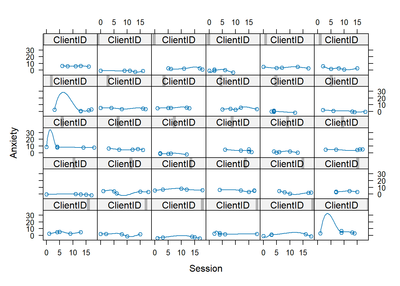
xyplot(Anxiety ~ Index | ClientID, data = RndmLong, prepanel = function(x,
    y) prepanel.loess(x, y, family = "gaussian"), xlab = "Index", ylab = "Anxiety",
    panel = function(x, y) {
        panel.xyplot(x, y)
        panel.loess(x, y, family = "gaussian")
    }, as.table = T)
When we examine these, we simply look for patterns:
- Are there general trends?
- Seems like anxiety tends to go downward
- Are the levels at the start of the study (Wave 1, intercept) at the same place? Or differenct?
- In this dataset, they are definitely different.
- Is the change-over-time (slope) linear or curvilinear?
- The general trend seems to be linear – a decline or staying flat
- Some show “bump ups” in anxiety before it declines again
- One case shows a “bump down” in anxiety and then it rises again
Because clients (a) start at different points and (b) change differently, MLM is a reasonable approach to analyzing the data. Our choice of L1 (time-covarying) and L2 (person-level) variables may help disentangle these differences.
As we continue the preliminary exploration, I will use the Session0 variable as our representation of time because it is “truer” to the data.
13.5.5.2 Parametric Smoothing of the Empirical Growth Trajectory w OLS Regression**
Here we fit a separate parametric model to each person’s data; OLS is appropriate for this preliminary exploration. Next we can summarize each person’s growth trajectory by fitting a separate parametric model to each person’s data. Singer and Willett (2003) indicate that this is “hardly the most efficient use of longitudinal data…[but] it connects empirical researchers with their data in a direct and intimate way” (p. 28).
We must identify a “common functional form” (e.g., linear, quadratic, cubic) to fit to all the individuals. Clearly, this is an oversimplification. However, it allows us to easily spot folks for whom the model works and does not. Often the best choice is a straight line and that’s what we will do here.
There are three steps:
- Estimate a within-person regression model for each person. This means we regress the outcome [Anxiety] on some representation of time(we’ll use Session0 around 0). In order to conduct separate analyses for each person, we conduct the regression analysis “by Client”
- Use summary statistics from all the within-person regression models into a separate data set. For a linear change model, the intercept and slope summarize their growth trajectory; the \(R^2\) and residual variance statistics summarize the goodness of fit.
- Superimpose each person’s fitted regression line on a plot of their empirical growth record.
Let’s start with step #1:
This little script produces individual regression models for each person.
ANX_OLS <- function(RndmLong) {
    summary(lm(Anxiety ~ Session0, data = RndmLong))
}
by(RndmLong, RndmLong$ClientID, ANX_OLS)
## RndmLong$ClientID: 175
##
## Call:
## lm(formula = Anxiety ~ Session0, data = RndmLong)
##
## Residuals:
## 1 2 3 4 5
## 0.05038 -0.29755 0.08804 0.47882 -0.31968
##
## Coefficients:
## Estimate Std. Error t value Pr(>|t|)
## (Intercept) 6.75056 0.54322 12.427 0.00112 **
## Session0 -0.07347 0.04779 -1.537 0.22181
## ---
## Signif. codes: 0 '***' 0.001 '**' 0.01 '*' 0.05 '.' 0.1 ' ' 1
##
## Residual standard error: 0.3787 on 3 degrees of freedom
## Multiple R-squared: 0.4407, Adjusted R-squared: 0.2542
## F-statistic: 2.363 on 1 and 3 DF, p-value: 0.2218
##
## ------------------------------------------------------------
## RndmLong$ClientID: 343
##
## Call:
## lm(formula = Anxiety ~ Session0, data = RndmLong)
##
## Residuals:
## 6 7 8 9 10
## -0.1008 0.2721 0.6444 -1.1712 0.3555
##
## Coefficients:
## Estimate Std. Error t value Pr(>|t|)
## (Intercept) -0.49676 0.75416 -0.659 0.557
## Session0 -0.07398 0.06735 -1.098 0.352
##
## Residual standard error: 0.816 on 3 degrees of freedom
## Multiple R-squared: 0.2868, Adjusted R-squared: 0.04912
## F-statistic: 1.207 on 1 and 3 DF, p-value: 0.3523
##
## ------------------------------------------------------------
## RndmLong$ClientID: 755
##
## Call:
## lm(formula = Anxiety ~ Session0, data = RndmLong)
##
## Residuals:
## 11 12 13 14 15
## 0.2702 -0.5245 0.2561 0.9874 -0.9893
##
## Coefficients:
## Estimate Std. Error t value Pr(>|t|)
## (Intercept) 2.68707 0.92956 2.891 0.063 .
## Session0 -0.04112 0.07372 -0.558 0.616
## ---
## Signif. codes: 0 '***' 0.001 '**' 0.01 '*' 0.05 '.' 0.1 ' ' 1
##
## Residual standard error: 0.8883 on 3 degrees of freedom
## Multiple R-squared: 0.09397, Adjusted R-squared: -0.208
## F-statistic: 0.3112 on 1 and 3 DF, p-value: 0.6159
##
## ------------------------------------------------------------
## RndmLong$ClientID: 818
##
## Call:
## lm(formula = Anxiety ~ Session0, data = RndmLong)
##
## Residuals:
## 16 17 18 19 20
## -1.1235 -0.4274 1.1499 1.6847 -1.2837
##
## Coefficients:
## Estimate Std. Error t value Pr(>|t|)
## (Intercept) 0.2063 1.0700 0.193 0.859
## Session0 -0.2684 0.2140 -1.254 0.299
##
## Residual standard error: 1.555 on 3 degrees of freedom
## Multiple R-squared: 0.3439, Adjusted R-squared: 0.1253
## F-statistic: 1.573 on 1 and 3 DF, p-value: 0.2986
##
## ------------------------------------------------------------
## RndmLong$ClientID: 1435
##
## Call:
## lm(formula = Anxiety ~ Session0, data = RndmLong)
##
## Residuals:
## 21 22 23 24 25
## 0.5863 -0.9380 -0.3808 1.2743 -0.5418
##
## Coefficients:
## Estimate Std. Error t value Pr(>|t|)
## (Intercept) 4.29380 0.80645 5.324 0.0129 *
## Session0 -0.05622 0.07818 -0.719 0.5240
## ---
## Signif. codes: 0 '***' 0.001 '**' 0.01 '*' 0.05 '.' 0.1 ' ' 1
##
## Residual standard error: 1.047 on 3 degrees of freedom
## Multiple R-squared: 0.147, Adjusted R-squared: -0.1373
## F-statistic: 0.5171 on 1 and 3 DF, p-value: 0.524
##
## ------------------------------------------------------------
## RndmLong$ClientID: 1540
##
## Call:
## lm(formula = Anxiety ~ Session0, data = RndmLong)
##
## Residuals:
## 26 27 28 29 30
## 1.8238 -1.7020 0.0878 -1.4607 1.2512
##
## Coefficients:
## Estimate Std. Error t value Pr(>|t|)
## (Intercept) 4.6373 1.6804 2.760 0.0702 .
## Session0 -0.2185 0.1838 -1.189 0.3199
## ---
## Signif. codes: 0 '***' 0.001 '**' 0.01 '*' 0.05 '.' 0.1 ' ' 1
##
## Residual standard error: 1.819 on 3 degrees of freedom
## Multiple R-squared: 0.3203, Adjusted R-squared: 0.09379
## F-statistic: 1.414 on 1 and 3 DF, p-value: 0.3199
##
## ------------------------------------------------------------
## RndmLong$ClientID: 2039
##
## Call:
## lm(formula = Anxiety ~ Session0, data = RndmLong)
##
## Residuals:
## 31 32 33 34 35
## 0.5442 -1.1692 -0.6984 -0.1480 1.4715
##
## Coefficients:
## Estimate Std. Error t value Pr(>|t|)
## (Intercept) 2.09163 1.44704 1.445 0.244
## Session0 -0.02286 0.10834 -0.211 0.846
##
## Residual standard error: 1.203 on 3 degrees of freedom
## Multiple R-squared: 0.01463, Adjusted R-squared: -0.3138
## F-statistic: 0.04454 on 1 and 3 DF, p-value: 0.8464
##
## ------------------------------------------------------------
## RndmLong$ClientID: 2578
##
## Call:
## lm(formula = Anxiety ~ Session0, data = RndmLong)
##
## Residuals:
## 36 37 38 39 40
## 0.1239 0.3173 -0.7597 0.6067 -0.2881
##
## Coefficients:
## Estimate Std. Error t value Pr(>|t|)
## (Intercept) 5.11349 0.46553 10.984 0.00162 **
## Session0 -0.08044 0.04164 -1.932 0.14889
## ---
## Signif. codes: 0 '***' 0.001 '**' 0.01 '*' 0.05 '.' 0.1 ' ' 1
##
## Residual standard error: 0.6176 on 3 degrees of freedom
## Multiple R-squared: 0.5544, Adjusted R-squared: 0.4058
## F-statistic: 3.732 on 1 and 3 DF, p-value: 0.1489
##
## ------------------------------------------------------------
## RndmLong$ClientID: 2983
##
## Call:
## lm(formula = Anxiety ~ Session0, data = RndmLong)
##
## Residuals:
## 41 42 43 44 45
## -0.16092 0.14607 0.03212 0.53772 -0.55499
##
## Coefficients:
## Estimate Std. Error t value Pr(>|t|)
## (Intercept) 5.127752 0.399302 12.842 0.00102 **
## Session0 0.009937 0.046107 0.216 0.84319
## ---
## Signif. codes: 0 '***' 0.001 '**' 0.01 '*' 0.05 '.' 0.1 ' ' 1
##
## Residual standard error: 0.4638 on 3 degrees of freedom
## Multiple R-squared: 0.01525, Adjusted R-squared: -0.313
## F-statistic: 0.04644 on 1 and 3 DF, p-value: 0.8432
##
## ------------------------------------------------------------
## RndmLong$ClientID: 3600
##
## Call:
## lm(formula = Anxiety ~ Session0, data = RndmLong)
##
## Residuals:
## 46 47 48 49 50
## -0.29675 0.03494 -0.97922 1.89035 -0.64932
##
## Coefficients:
## Estimate Std. Error t value Pr(>|t|)
## (Intercept) 3.39206 1.52325 2.227 0.112
## Session0 0.04242 0.13288 0.319 0.771
##
## Residual standard error: 1.297 on 3 degrees of freedom
## Multiple R-squared: 0.03285, Adjusted R-squared: -0.2895
## F-statistic: 0.1019 on 1 and 3 DF, p-value: 0.7705
##
## ------------------------------------------------------------
## RndmLong$ClientID: 3748
##
## Call:
## lm(formula = Anxiety ~ Session0, data = RndmLong)
##
## Residuals:
## 51 52 53 54 55
## -0.45080 0.93546 0.09437 -0.52268 -0.05635
##
## Coefficients:
## Estimate Std. Error t value Pr(>|t|)
## (Intercept) 1.03581 0.57534 1.800 0.170
## Session0 -0.21264 0.09074 -2.343 0.101
##
## Residual standard error: 0.6742 on 3 degrees of freedom
## Multiple R-squared: 0.6467, Adjusted R-squared: 0.5289
## F-statistic: 5.491 on 1 and 3 DF, p-value: 0.1009
##
## ------------------------------------------------------------
## RndmLong$ClientID: 4017
##
## Call:
## lm(formula = Anxiety ~ Session0, data = RndmLong)
##
## Residuals:
## 56 57 58 59 60
## 0.26714 -0.15368 0.00644 -0.61559 0.49568
##
## Coefficients:
## Estimate Std. Error t value Pr(>|t|)
## (Intercept) 2.23595 0.45737 4.889 0.0164 *
## Session0 -0.16471 0.03788 -4.349 0.0225 *
## ---
## Signif. codes: 0 '***' 0.001 '**' 0.01 '*' 0.05 '.' 0.1 ' ' 1
##
## Residual standard error: 0.4898 on 3 degrees of freedom
## Multiple R-squared: 0.8631, Adjusted R-squared: 0.8174
## F-statistic: 18.91 on 1 and 3 DF, p-value: 0.02246
##
## ------------------------------------------------------------
## RndmLong$ClientID: 4488
##
## Call:
## lm(formula = Anxiety ~ Session0, data = RndmLong)
##
## Residuals:
## 61 62 63 64 65
## 0.001669 0.521712 -0.510843 -0.045551 0.033013
##
## Coefficients:
## Estimate Std. Error t value Pr(>|t|)
## (Intercept) 8.67916 0.29167 29.757 0.0000834 ***
## Session0 -0.05812 0.02776 -2.094 0.127
## ---
## Signif. codes: 0 '***' 0.001 '**' 0.01 '*' 0.05 '.' 0.1 ' ' 1
##
## Residual standard error: 0.4228 on 3 degrees of freedom
## Multiple R-squared: 0.5937, Adjusted R-squared: 0.4582
## F-statistic: 4.383 on 1 and 3 DF, p-value: 0.1273
##
## ------------------------------------------------------------
## RndmLong$ClientID: 4854
##
## Call:
## lm(formula = Anxiety ~ Session0, data = RndmLong)
##
## Residuals:
## 66 67 68 69 70
## 0.4984 -0.7896 -0.2480 0.8098 -0.2706
##
## Coefficients:
## Estimate Std. Error t value Pr(>|t|)
## (Intercept) 6.40250 0.80019 8.001 0.00407 **
## Session0 -0.11262 0.06997 -1.610 0.20586
## ---
## Signif. codes: 0 '***' 0.001 '**' 0.01 '*' 0.05 '.' 0.1 ' ' 1
##
## Residual standard error: 0.7444 on 3 degrees of freedom
## Multiple R-squared: 0.4634, Adjusted R-squared: 0.2845
## F-statistic: 2.591 on 1 and 3 DF, p-value: 0.2059
##
## ------------------------------------------------------------
## RndmLong$ClientID: 5320
##
## Call:
## lm(formula = Anxiety ~ Session0, data = RndmLong)
##
## Residuals:
## 71 72 73 74 75
## -0.4121 0.2233 -0.1676 0.5102 -0.1538
##
## Coefficients:
## Estimate Std. Error t value Pr(>|t|)
## (Intercept) -0.62417 0.33518 -1.862 0.1595
## Session0 -0.14753 0.05135 -2.873 0.0639 .
## ---
## Signif. codes: 0 '***' 0.001 '**' 0.01 '*' 0.05 '.' 0.1 ' ' 1
##
## Residual standard error: 0.421 on 3 degrees of freedom
## Multiple R-squared: 0.7334, Adjusted R-squared: 0.6445
## F-statistic: 8.253 on 1 and 3 DF, p-value: 0.0639
##
## ------------------------------------------------------------
## RndmLong$ClientID: 6114
##
## Call:
## lm(formula = Anxiety ~ Session0, data = RndmLong)
##
## Residuals:
## 76 77 78 79 80
## -0.04382 -0.32102 2.24396 -0.52170 -1.35743
##
## Coefficients:
## Estimate Std. Error t value Pr(>|t|)
## (Intercept) 6.3648 2.5328 2.513 0.0867 .
## Session0 -0.2398 0.1903 -1.260 0.2966
## ---
## Signif. codes: 0 '***' 0.001 '**' 0.01 '*' 0.05 '.' 0.1 ' ' 1
##
## Residual standard error: 1.555 on 3 degrees of freedom
## Multiple R-squared: 0.3462, Adjusted R-squared: 0.1283
## F-statistic: 1.589 on 1 and 3 DF, p-value: 0.2966
##
## ------------------------------------------------------------
## RndmLong$ClientID: 6407
##
## Call:
## lm(formula = Anxiety ~ Session0, data = RndmLong)
##
## Residuals:
## 81 82 83 84 85
## 0.6233 -0.9159 -0.1976 1.0334 -0.5433
##
## Coefficients:
## Estimate Std. Error t value Pr(>|t|)
## (Intercept) 1.78203 1.02976 1.731 0.182
## Session0 -0.07499 0.12379 -0.606 0.587
##
## Residual standard error: 0.9362 on 3 degrees of freedom
## Multiple R-squared: 0.109, Adjusted R-squared: -0.188
## F-statistic: 0.367 on 1 and 3 DF, p-value: 0.5874
##
## ------------------------------------------------------------
## RndmLong$ClientID: 6559
##
## Call:
## lm(formula = Anxiety ~ Session0, data = RndmLong)
##
## Residuals:
## 86 87 88 89 90
## 0.09503 -0.03545 -0.62788 0.27986 0.28844
##
## Coefficients:
## Estimate Std. Error t value Pr(>|t|)
## (Intercept) 4.49464 0.44869 10.017 0.00212 **
## Session0 0.01978 0.03487 0.567 0.61016
## ---
## Signif. codes: 0 '***' 0.001 '**' 0.01 '*' 0.05 '.' 0.1 ' ' 1
##
## Residual standard error: 0.4344 on 3 degrees of freedom
## Multiple R-squared: 0.0969, Adjusted R-squared: -0.2041
## F-statistic: 0.3219 on 1 and 3 DF, p-value: 0.6102
##
## ------------------------------------------------------------
## RndmLong$ClientID: 7142
##
## Call:
## lm(formula = Anxiety ~ Session0, data = RndmLong)
##
## Residuals:
## 91 92 93 94 95
## -0.2880 0.5761 0.2737 0.1724 -0.7343
##
## Coefficients:
## Estimate Std. Error t value Pr(>|t|)
## (Intercept) -0.06634 0.56654 -0.117 0.914
## Session0 -0.05314 0.04468 -1.189 0.320
##
## Residual standard error: 0.5941 on 3 degrees of freedom
## Multiple R-squared: 0.3205, Adjusted R-squared: 0.09396
## F-statistic: 1.415 on 1 and 3 DF, p-value: 0.3198
##
## ------------------------------------------------------------
## RndmLong$ClientID: 7767
##
## Call:
## lm(formula = Anxiety ~ Session0, data = RndmLong)
##
## Residuals:
## 96 97 98 99 100
## 1.0376 0.6314 -2.2630 0.4364 0.1577
##
## Coefficients:
## Estimate Std. Error t value Pr(>|t|)
## (Intercept) 3.61480 1.16058 3.115 0.0527 .
## Session0 -0.03206 0.10499 -0.305 0.7801
## ---
## Signif. codes: 0 '***' 0.001 '**' 0.01 '*' 0.05 '.' 0.1 ' ' 1
##
## Residual standard error: 1.507 on 3 degrees of freedom
## Multiple R-squared: 0.03014, Adjusted R-squared: -0.2931
## F-statistic: 0.09323 on 1 and 3 DF, p-value: 0.7801
##
## ------------------------------------------------------------
## RndmLong$ClientID: 9066
##
## Call:
## lm(formula = Anxiety ~ Session0, data = RndmLong)
##
## Residuals:
## 101 102 103 104 105
## -0.8117 0.1204 1.3825 0.2906 -0.9818
##
## Coefficients:
## Estimate Std. Error t value Pr(>|t|)
## (Intercept) 6.46252 0.82127 7.869 0.00428 **
## Session0 0.01625 0.07645 0.213 0.84533
## ---
## Signif. codes: 0 '***' 0.001 '**' 0.01 '*' 0.05 '.' 0.1 ' ' 1
##
## Residual standard error: 1.1 on 3 degrees of freedom
## Multiple R-squared: 0.01483, Adjusted R-squared: -0.3136
## F-statistic: 0.04516 on 1 and 3 DF, p-value: 0.8453
##
## ------------------------------------------------------------
## RndmLong$ClientID: 9097
##
## Call:
## lm(formula = Anxiety ~ Session0, data = RndmLong)
##
## Residuals:
## 106 107 108 109 110
## 0.1710 0.1344 -1.4475 0.3723 0.7698
##
## Coefficients:
## Estimate Std. Error t value Pr(>|t|)
## (Intercept) 6.7369 1.2504 5.388 0.0125 *
## Session0 -0.1322 0.0901 -1.468 0.2385
## ---
## Signif. codes: 0 '***' 0.001 '**' 0.01 '*' 0.05 '.' 0.1 ' ' 1
##
## Residual standard error: 0.9787 on 3 degrees of freedom
## Multiple R-squared: 0.4179, Adjusted R-squared: 0.2239
## F-statistic: 2.154 on 1 and 3 DF, p-value: 0.2385
##
## ------------------------------------------------------------
## RndmLong$ClientID: 9814
##
## Call:
## lm(formula = Anxiety ~ Session0, data = RndmLong)
##
## Residuals:
## 111 112 113 114 115
## 1.5780 -0.1342 -2.2272 0.2243 0.5592
##
## Coefficients:
## Estimate Std. Error t value Pr(>|t|)
## (Intercept) 3.8789 1.9063 2.035 0.135
## Session0 -0.1239 0.1495 -0.829 0.468
##
## Residual standard error: 1.616 on 3 degrees of freedom
## Multiple R-squared: 0.1864, Adjusted R-squared: -0.08483
## F-statistic: 0.6872 on 1 and 3 DF, p-value: 0.4679
##
## ------------------------------------------------------------
## RndmLong$ClientID: 9998
##
## Call:
## lm(formula = Anxiety ~ Session0, data = RndmLong)
##
## Residuals:
## 116 117 118 119 120
## 0.3646 -0.8017 1.1655 -0.5472 -0.1813
##
## Coefficients:
## Estimate Std. Error t value Pr(>|t|)
## (Intercept) 3.40739 1.32511 2.571 0.0824 .
## Session0 0.01101 0.11264 0.098 0.9283
## ---
## Signif. codes: 0 '***' 0.001 '**' 0.01 '*' 0.05 '.' 0.1 ' ' 1
##
## Residual standard error: 0.9067 on 3 degrees of freedom
## Multiple R-squared: 0.003173, Adjusted R-squared: -0.3291
## F-statistic: 0.00955 on 1 and 3 DF, p-value: 0.9283
##
## ------------------------------------------------------------
## RndmLong$ClientID: 10398
##
## Call:
## lm(formula = Anxiety ~ Session0, data = RndmLong)
##
## Residuals:
## 121 122 123 124 125
## -1.1381 0.9662 1.3901 -1.5399 0.3217
##
## Coefficients:
## Estimate Std. Error t value Pr(>|t|)
## (Intercept) 3.53102 1.21714 2.901 0.0624 .
## Session0 0.07828 0.15927 0.491 0.6568
## ---
## Signif. codes: 0 '***' 0.001 '**' 0.01 '*' 0.05 '.' 0.1 ' ' 1
##
## Residual standard error: 1.487 on 3 degrees of freedom
## Multiple R-squared: 0.07452, Adjusted R-squared: -0.234
## F-statistic: 0.2416 on 1 and 3 DF, p-value: 0.6568
##
## ------------------------------------------------------------
## RndmLong$ClientID: 11153
##
## Call:
## lm(formula = Anxiety ~ Session0, data = RndmLong)
##
## Residuals:
## 126 127 128 129 130
## 0.3641 0.1975 0.4548 -2.2425 1.2261
##
## Coefficients:
## Estimate Std. Error t value Pr(>|t|)
## (Intercept) 1.9946 1.1061 1.803 0.169
## Session0 -0.1025 0.1248 -0.821 0.472
##
## Residual standard error: 1.518 on 3 degrees of freedom
## Multiple R-squared: 0.1836, Adjusted R-squared: -0.08852
## F-statistic: 0.6747 on 1 and 3 DF, p-value: 0.4716
##
## ------------------------------------------------------------
## RndmLong$ClientID: 11639
##
## Call:
## lm(formula = Anxiety ~ Session0, data = RndmLong)
##
## Residuals:
## 131 132 133 134 135
## -0.5633 0.3197 1.2701 0.3633 -1.3898
##
## Coefficients:
## Estimate Std. Error t value Pr(>|t|)
## (Intercept) -3.35216 0.94537 -3.546 0.0382 *
## Session0 0.01803 0.07878 0.229 0.8337
## ---
## Signif. codes: 0 '***' 0.001 '**' 0.01 '*' 0.05 '.' 0.1 ' ' 1
##
## Residual standard error: 1.169 on 3 degrees of freedom
## Multiple R-squared: 0.01716, Adjusted R-squared: -0.3104
## F-statistic: 0.05239 on 1 and 3 DF, p-value: 0.8337
##
## ------------------------------------------------------------
## RndmLong$ClientID: 11713
##
## Call:
## lm(formula = Anxiety ~ Session0, data = RndmLong)
##
## Residuals:
## 136 137 138 139 140
## 0.27002 1.08393 -1.06589 -0.38107 0.09301
##
## Coefficients:
## Estimate Std. Error t value Pr(>|t|)
## (Intercept) 2.46789 0.63760 3.871 0.0305 *
## Session0 -0.02542 0.07165 -0.355 0.7462
## ---
## Signif. codes: 0 '***' 0.001 '**' 0.01 '*' 0.05 '.' 0.1 ' ' 1
##
## Residual standard error: 0.9197 on 3 degrees of freedom
## Multiple R-squared: 0.04028, Adjusted R-squared: -0.2796
## F-statistic: 0.1259 on 1 and 3 DF, p-value: 0.7462
##
## ------------------------------------------------------------
## RndmLong$ClientID: 12081
##
## Call:
## lm(formula = Anxiety ~ Session0, data = RndmLong)
##
## Residuals:
## 141 142 143 144 145
## -1.4042 0.8308 0.6680 1.3966 -1.4913
##
## Coefficients:
## Estimate Std. Error t value Pr(>|t|)
## (Intercept) 0.385038 1.021952 0.377 0.731
## Session0 -0.001875 0.093447 -0.020 0.985
##
## Residual standard error: 1.558 on 3 degrees of freedom
## Multiple R-squared: 0.0001342, Adjusted R-squared: -0.3332
## F-statistic: 0.0004026 on 1 and 3 DF, p-value: 0.9853
##
## ------------------------------------------------------------
## RndmLong$ClientID: 12409
##
## Call:
## lm(formula = Anxiety ~ Session0, data = RndmLong)
##
## Residuals:
## 146 147 148 149 150
## -0.715243 2.248873 -0.389445 0.001022 -1.145207
##
## Coefficients:
## Estimate Std. Error t value Pr(>|t|)
## (Intercept) 3.95251 1.53686 2.572 0.0824 .
## Session0 0.02669 0.14956 0.178 0.8697
## ---
## Signif. codes: 0 '***' 0.001 '**' 0.01 '*' 0.05 '.' 0.1 ' ' 1
##
## Residual standard error: 1.531 on 3 degrees of freedom
## Multiple R-squared: 0.01051, Adjusted R-squared: -0.3193
## F-statistic: 0.03185 on 1 and 3 DF, p-value: 0.8697Looking at our data, we might observe:
- \(R^2\) values range from 0 to 74%
- Level of anxiety starts at different places
- For many, anxiety decreases as a function of session
- but not for all,
- and for a few it goes negative
Next we superimpose each client’s fitted OLS trajectory on their empirical growth plot.
xyplot(Anxiety ~ Session0 | ClientID, data = RndmLong, panel = function(x,
    y) {
    panel.xyplot(x, y)
    panel.lmline(x, y)
}, as.table = T)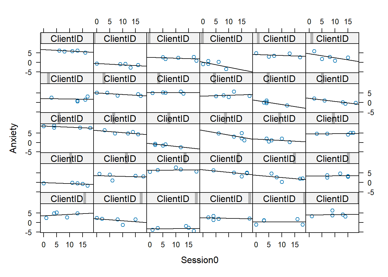
What do we observe? A linear change trajectory
- is ideal for a few members
- reasonable for many others
- The \(R^2\) coincides well with those for whom the line is the best fit
Singer and Willett (2003) can read your minds, “Don’t OLS regression methods assume independence and homoscedastic residuals?” Why, yes! They do. Singer and Willett indicate OLS estimates are very useful for exploratory purposes in that they provide an unbiased estimate of the intercept and slope of the individual change.
13.5.5.3 Snapshot of the Entire Set of Smooth Trajectories**
We can plop all our trajectories in a set of smoothed individual trajectories. This first plot is simply the raw data. This first plot is just a smoothed (there is a line for each client) plot of the raw/natural metric of the data.
# plot of raw data for every case Session0 provided splotchy data;
# Index0 gives some indication of change
interaction.plot(RndmLong$Index, RndmLong$ClientID, RndmLong$Anxiety)
The next two sets of code plot our fitted trajectories into a single plot.
First, we fit the model.
# fitting the linear model by ID
fit <- by(RndmLong, RndmLong$ClientID, function(bydata) fitted.values(lm(Anxiety ~
    Session0, data = bydata)))
fit <- unlist(fit)
Then make the plot.
# plotting the linear fit by ID
interaction.plot(RndmLong$Index, RndmLong$ClientID, fit, xlab = "Sessions",
    ylab = "Anxiety")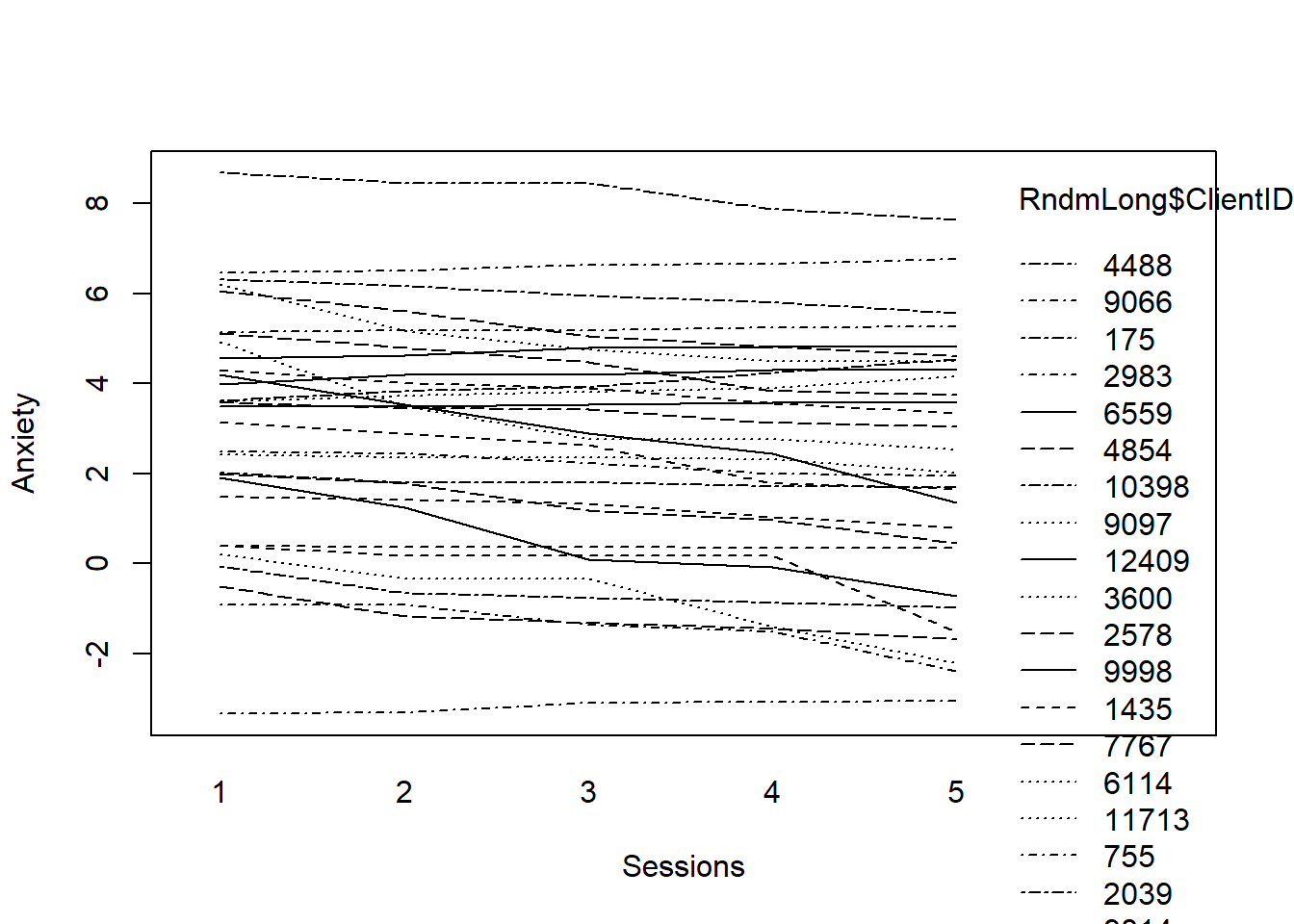
What do we observe? Clients present with varying levels of anxiety. On average, change in anxiety declined (at least a little) from the first wave to the fifth.
13.5.6 Examining intercepts, slopes, and their relationship
Sample means of the estimated intercepts and slopes (level-1 OLS estimated intercepts and slopes) are unbiased estimates of initial status and rate of change for each person. Their sample means are, therefore, unbiased estimates of the key features of the average observed change trajectory.
Sample variances (SDs) of the estimated intercepts and slopes quantify the amount of observed interindividual heterogeneity in change.
# obtaining the intercept from the linear model by ClientID
ints <- by(RndmLong, RndmLong$ClientID, function(data) coefficients(lm(Anxiety ~
    Session0, data = data))[[1]])
ints1 <- unlist(ints)
names(ints1) <- NULL
mean(ints1)
## [1] 3.239564## [1] 2.688367Our calculations tell us that at Session 1, anxiety is 3.23 (SD = 2.69).
The next two values calculate the slope and its variation.
# obtaining the slopes from linear model by id
slopes <- by(RndmLong, RndmLong$ClientID, function(data) coefficients(lm(Anxiety ~
    Session0, data = data))[[2]])
slopes1 <- unlist(slopes)
names(slopes1) <- NULL
mean(slopes1)
## [1] -0.06980594## [1] 0.08853341Here we learn that the average slope is -0.07 (SD = 0.08). On average, anxiety decreases by .07 points per session. Relative to their means, the magnitudes of the SDs around the slope and intercept are pretty big, so there is a great deal of variation.
Sample correlation between the estimated intercepts and slopes summarizes the association between the fitted initial status and fitted rate of change. It answers the question, “Are observed initial status and rate of change related?”
## [1] 0.008575535Not really. r = 0.01.
13.5.7 Exploring the relationship between Change and Time-Invariant Predictors
Looking at our level-2 predictors can help uncover systematic interindividual differences in change. In this vignette religious affiliation and sexual identity are our L2 predictors.
Let’s start with religious affiliation Is there a difference in intercept (initial tolerance) or slope (rate of change) as a function of religious affiliation?
We start by selecting DR, fitting a regression model, and plotting it.
# fitting the linear model by ID, DR only
DR <- filter(RndmLong, DRel0 == "0")
fitmlist <- by(DR, DR$ClientID, function(bydata) fitted.values(lm(Anxiety ~
    Session0, data = bydata)))
fitDR <- unlist(fitmlist)
# appending the average for the whole group of DR
lm.DR <- fitted(lm(Anxiety ~ Session0, data = DR))
names(lm.DR) <- NULL
fit.DR2 <- c(fitDR, lm.DR[1:5])
Sess1.DR <- c(DR$Index, seq(1, 5)) #Note that I used Session0 to create the lm, but plotted by Index0
id.DR <- c(DR$ClientID, rep(30, 5))# plotting the linear fit by id, males id.m=111 denotes the average
# value for males
interaction.plot(Sess1.DR, id.DR, fit.DR2, ylim = c(-2, 8), xlab = "Sessions",
ylab = "Anxiety", lwd = 1)
title(main = "Dominant Religious")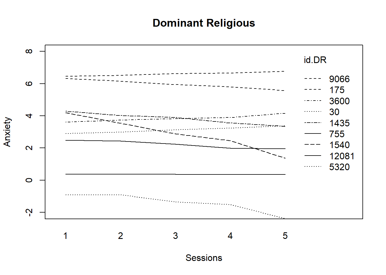 Trajectories for those from dominantreligions stay flat; a few decline.
Now for non-dominant religious (including those that are affiliated and unaffiliated).
# fitting the linear model by ID, DR only
NDR <- filter(RndmLong, DRel0 == "1")
fitmlist <- by(NDR, NDR$ClientID, function(bydata) fitted.values(lm(Anxiety ~
    Session0, data = bydata)))
fitNDR <- unlist(fitmlist)
# appending the average for the whole group of males
lm.NDR <- fitted(lm(Anxiety ~ Session0, data = NDR))
names(lm.NDR) <- NULL
fit.NDR2 <- c(fitNDR, lm.NDR[1:5])
Sess1.NDR <- c(NDR$Index, seq(1, 5)) #Note that I used Session0 to create the lm, but plotted by Index0
id.NDR <- c(NDR$ClientID, rep(30, 5))# plotting the linear fit by id, males id.m=111 denotes the average
# value for males
interaction.plot(Sess1.NDR, id.NDR, fit.NDR2, ylim = c(-2, 8), xlab = "Sessions",
ylab = "Anxiety", lwd = 1)
title(main = "Non-Dominant Religious")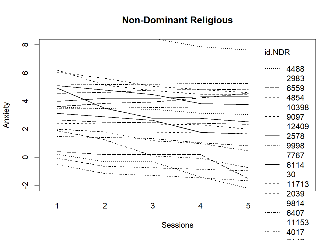
It appears that there is more decline in anxiety for those who claim non-dominant religions.
What about the effects of sexual identity?
# fitting the linear model by ID, HET = 0 only
HET <- filter(RndmLong, Het0 == "0")
fitmlist <- by(HET, HET$ClientID, function(bydata) fitted.values(lm(Anxiety ~
    Session0, data = bydata)))
fitHET <- unlist(fitmlist)
# appending the average for the whole group of males
lm.HET <- fitted(lm(Anxiety ~ Session0, data = HET))
names(lm.HET) <- NULL
fit.HET <- c(fitHET, lm.HET[1:5])
Sess1.HET <- c(HET$Index, seq(1, 5)) #Note that I used Session0 to create the lm, but plotted by Index0
id.HET <- c(HET$ClientID, rep(30, 5))# plotting the linear fit by id, males id.m=111 denotes the average
# value for males
interaction.plot(Sess1.HET, id.HET, fit.HET, ylim = c(-2, 8), xlab = "Sessions",
ylab = "Anxiety", lwd = 1)
title(main = "Heterosexual")
Among clients who identify as heterosexual, there is a mixed profile. Clients start with varying degrees of anxiety and we see it stay the same, increase, and decrease.
# fitting the linear model by ID, DR only
LGBQQ <- filter(RndmLong, Het0 == "1")
fitmlist <- by(LGBQQ, LGBQQ$ClientID, function(bydata) fitted.values(lm(Anxiety ~
    Session0, data = bydata)))
fitLGBQQ <- unlist(fitmlist)
# appending the average for the whole group of males
lm.LGBQQ <- fitted(lm(Anxiety ~ Session0, data = LGBQQ))
names(lm.LGBQQ) <- NULL
fit.LGBQQ <- c(fitLGBQQ, lm.LGBQQ[1:5])
Sess1.LGBQQ <- c(LGBQQ$Index, seq(1, 5)) #Note that I used Session0 to create the lm, but plotted by Index0
id.LGBQQ <- c(LGBQQ$ClientID, rep(30, 5))# plotting the linear fit by id, males id.m=111 denotes the average
# value for males
interaction.plot(Sess1.LGBQQ, id.LGBQQ, fit.LGBQQ, ylim = c(-2, 8), xlab = "Sessions",
ylab = "Anxiety", lwd = 1)
title(main = "LGBQQ")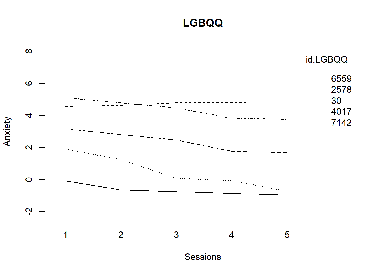
What do we observe? Clients who identify as LGBQQ start at different levels of anxiety; most decline somewhere in the middle and then maintain in a consistent/level manner.
13.5.8 The Relationship between OLS-Estimated Trajectories and Substantive Predictors
Below are two plots (and corresponding correlation coefficients) for religious affiliation and sexual identity regarding intercept (or initial status). They help us answer the question, is initial status different as a function of gender (then, exposure level).
NOTE that these are calculated from the the wide-format.
First, is anxiety at Session0 (our initial, or intercept) different for those from dominant and nondominant religions?
For these analyses of intercepts, the fitted model that we are using for the plot and correlation keeps the assessment at the Session0 intercept.
# Using the slopes and intercepts from the linear model fitted by id
# generated for use in table 2.3
plot(RndmSmpl30$DRel0, ints1, xlab = "Religion", ylab = "Fitted initial status")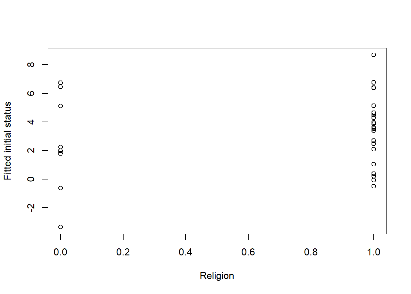
## [1] 0.1587707For religion, looking at the dots on 0 and 1 and the correlation, it looks like the anxiety intercept is lower for those from the dominant religion.
Next, is Anxiety at Session 1 different as a function of level of sexual identity?
 The plot of this random sample of data emphasizes that those who identify as LGBQQ are, proportionately, much smaller. Their range of anxiety is more restricted, but higher.
## [1] 0.1309987Looking at the correlation of intercepts and plot together, wee see that anxiety is higher for those who identify as LGBQQ.
Next, we look at 2 more plots and correlations for religion and sexual identity regarding slope/rate of change.
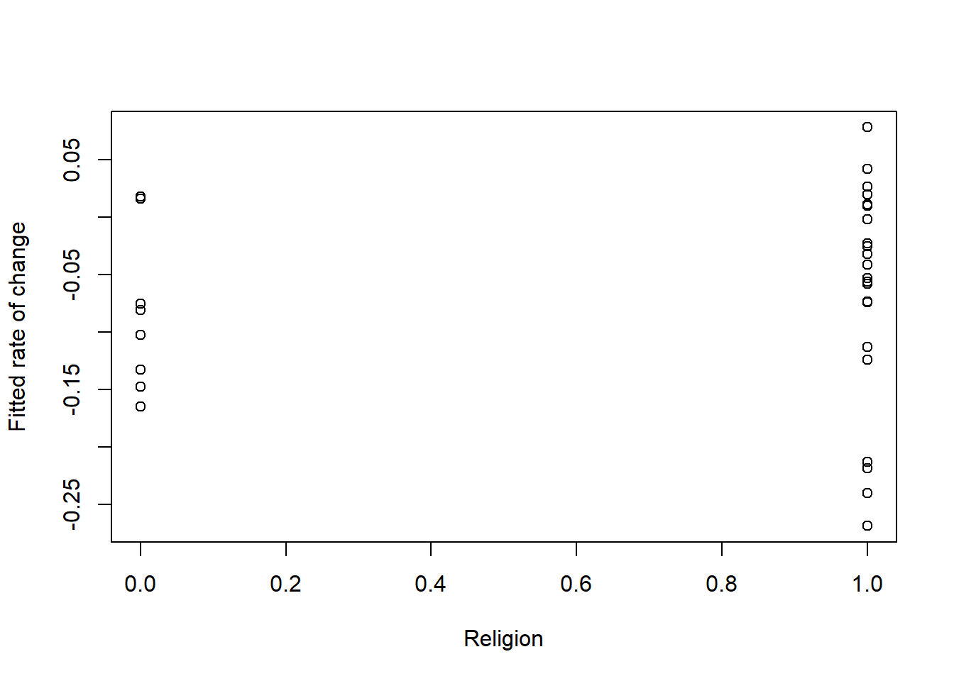
## [1] 0.09496023The plot is the rate of change or slope. It’s maybe a little more difficult to plot. We see that dominant religions have a slower rate of change than those who claim a nondominant religion (or no religion).
What about change in anxiety as a function of sexual identity?
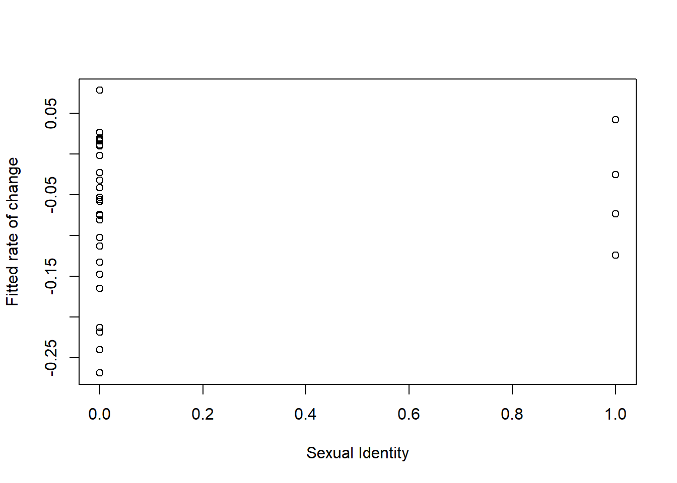
## [1] 0.1113146Those with who identify as LGBQQ have sharper rates of change.
13.5.9 APA Style Writeup
Method/Analytic Strategy
COMING SOON: Will be completed in next lesson
Results
Preliminary Analyses
Preliminary analysis involved the creation and visual inspection of empirical growth plots with parametrical and nonparmetrical smoothing. We also calculated and plotted intercepts, slopes, and their relationship. Results suggested that intercepts and slopes differed across the clients. Thus, utilizing multi-level modeling as the framework for analyzing the data is justified.
Primary Analyses
COMING SOON: Will be completed as we work the problem in the next lesson(s).
13.7 Practice Problems
The assignment is designed to span several lessons. Therefore, at this stage, please select a longitudinal dataset that will allow you to engage in the preliminary exploring, model building (including both exploration of an unconditional growth model and adding at least one L2 variables), and writing up a complete multilevel model for change (as specified below). Minimally, you should have a time-changing dependent variable and corresponding time-covarying (L1) predictor with a minimum of three waves each; our time-covarying predictor is Session. Variables will be clocked with a “sensible time metric.” You should also have a time invariant L2 predictor.
FROM THIS LESSON
- Restructure the dataset from wide to long.
- Provide three examples of data exploration
- An unfitted model
- A model fitted with a linear growth trajectory
- The fitted (or unfitted) data identified by the L2 predictor
FROM SUBSEQUENT LESSONS
- Using a staged approach to model development, report on at least four models, these must include
- An unconditional means model
- An unconditional growth model
- An intermediary model (please test both a time variable and an L2 variable)
- A final model
- Write up the Results as demonstrated in the lecture
- Table (use the tab_model outfile) and Figure are required
13.7.1 Problem #1: Rework the research vignette as demonstrated, but change the random seed
If this topic feels a bit overwhelming, simply change the random seed in the data simulation, then rework the problem. This should provide minor changes to the data (maybe in the second or third decimal point), but the results will likely be very similar.
13.7.2 Problem #2: Rework the research vignette using a different outcome variable
At the end of the lesson there is code that simulates data when depression is the outcome variable.
13.7.3 Problem #3: Use other data that is available to you
Using data for which you have permission and access (e.g., IRB approved data you have collected or from your lab; data you simulate from a published article; data from an open science repository; data from other chapters in this OER), complete the exploratory analyses.
13.7.4 Grading Rubric
Regardless of your choic(es) complete all the elements listed in the grading rubric.
| Assignment Component | ||
|---|---|---|
| 1. Identify and describe the variables in the model; there should be a time-varying DV and predictor as well as an L2 predictor | 5 | _____ |
| 2. Import the data and format the variables in the model | 5 | _____ |
| 3. Restructure the dataset from wide to long (or from long to wide) | 5 | _____ |
| 4. Produce multilevel descriptive statistics and correlation matrix | 5 | _____ |
| 5. Explore data with an unfitted model | 5 | _____ |
| 6. Explore data with a model fitted with a linear growth trajectory | 5 | _____ |
| 7. Explore data with the fitted (or unfitted) data identified by the L2 predictor | 5 | _____ |
| 8. Provide a write-up of what you found in this process | 5 | _____ |
| 9. Explanation to grader | 5 | _____ |
| Totals | 45 | _____ |
13.8 Simulated Data when Depression is the Outcome
One suggestion for practice is to work the second MLM example in the Lefevor et al. (Lefevor et al., 2017) example. The code below will simulate the data.
set.seed(200513)
n_client = 12825
n_session = 5
b0 = 1.84  #intercept for depression
b1 = -0.28  #b weight for L1 session
b2 = 0.15  #b weight for L2 sexual identity
b3 = -0.06  #b weight for L2 Rel1 (D-R vs ND-R & ND-U)
b4 = 0.04  #b weight for the L2 Rel2 (ND-R vs ND-U)
# the values used below are the +/- 3SD they produce continuous
# variables which later need to be transformed to categorical ones;
# admittedly this introduces a great deal of error/noise into the
# simulation the article didn't include a correlation matrix or M/SDs
# so this was a clunky process
(Session = runif(n_client * n_session, -3.67, 3.12))  #calc L1 Session, values are the +/3 3SD
(SexualIdentity = rep(runif(n_session, -6.64, 6.94), each = n_session))  #calc L2 Sexual Identity, values are the +/3 3SD
(Religion1 = rep(runif(n_session, -3.46, 3.34), each = n_session))  #calc L2 Religion1, values are the +/3 3SD
(Religion2 = rep(runif(n_session, -3.44, 3.36), each = n_session))  #calc L2 Religion2, values are the +/3 3SD
mu = 1.49  #intercept of empty model
sds = 2.264  #this is the SD of the DV
sd = 1  #this is the observation-level random effect variance that we set at 1

# ( church = rep(LETTERS[1:n_church], each = n_mbrs) ) #this worked
# in the prior
(client = rep(LETTERS[1:n_client], each = n_session))
# ( session = numbers[1:(n_client*n_session)] )
(clienteff = rnorm(n_client, 0, sds))
(clienteff = rep(clienteff, each = n_session))
(sessioneff = rnorm(n_client * n_session, 0, sd))
(Depression = b0 + b1 * Session + b2 * SexualIdentity + b3 * Religion1 +
    b4 * Religion2 + clienteff + sessioneff)
(dat = data.frame(client, clienteff, sessioneff, Session, SexualIdentity,
    Religion1, Religion2, Depression))

library(dplyr)
dat <- dat %>%
    mutate(ID = row_number())
# moving the ID number to the first column; requires
dat <- dat %>%
    select(ID, everything())

Lefevor2017D <- dat %>%
    select(ID, client, Session, SexualIdentity, Religion1, Religion2, Depression)

Lefevor2017D$ClientID <- rep(c(1:12825), each = 5)
# rounded Sexual Identity into dichotomous variable 85% were
# heterosexual,

# Rel2 has contrast codes for dominant religion (DR, 0), nondominant
# religious (NDR, 1) and nondominant unspecified (NDU, -1) Strategy
# is to figure out the raw score associated with the percentile rank
# of -1 and 0, to set the breakpoints for the coding NDU coded as -1
# 19.2+13.5+9.6 NDU has bottom 42.3 percent

# DR coded as 0, so quantile cut will be 42.3 + 52.7 = 95th 33.4 +
# 19.3 52.7% of sample (according to article) was DR must look up
# percentile ranks for 5% and 57.5%

# NDR 2.3+1+1+.7 NDR has 5% of sample 42.3+52.7
quantile(Lefevor2017D$Religion2, probs = c(0.423, 0.95))
# effects coding the second Religion variable so that NDU = -1, DR =
# 0, NDR = 1
Lefevor2017D$Rel2L2 <- ifelse(Lefevor2017D$Religion2 <= -0.3304528, -1,
    ifelse(Lefevor2017D$Religion2 >= -0.3304529 & Lefevor2017D$Religion2 <=
        2.4446784, 0, 1))

# creating the religion variable where DR is 0 and NDR and NDU are
# both 1
Lefevor2017D$DRel0 <- plyr::mapvalues(Lefevor2017D$Rel2L2, from = c(-1,
    0, 1), to = c(1, 0, 1))
## The following `from` values were not present in `x`: 1# checking DRel0_table <- table(Lefevor2017D$DRel0)
# prop.table(DRel0_table) heterosexual is -1 LGBQQ is 1
# quantile(Lefevor2017D$SexualIdentity, probs = c(.85))
Lefevor2017D$SexID <- ifelse(Lefevor2017D$SexualIdentity <= 5.747946, -1,
1)
Lefevor2017D$Het0 <- plyr::mapvalues(Lefevor2017D$SexID, from = c(-1, 1),
to = c(0, 1))
# Het0_table <- table(Lefevor2017D$Het0) prop.table(Het0_table)#to
# make sure that 85% are coded 0 for Het
# creating a variable representing the session number for each
# client, in the article up to 20 sessions were allowed.
# install.packages('scales')
# Right from the beginning I centered this so that 0 would represent
# intake
Lefevor2017D$Session0 <- as.integer(scales::rescale(Lefevor2017D$Session,
to = c(0, 19)))
# creating session waves (1 thru 5) by rank ordering within each
# person's variable the continuous variable Session that was created
# in the original simulation
Lefevor2017D <- Lefevor2017D %>%
dplyr::group_by(ClientID) %>%
dplyr::mutate(Index = rank(Session))
# selecting the simulated variables
Lefevor2017D_sim <- Lefevor2017D %>%
dplyr::select(ClientID, Index, Session0, Depression, DRel0, Het0)
# In the transition from long-to-wide, it seems like you can only do
# one L1 variable at a time When there are multiple L1 and L2 vars,
# put all L2 vars on left of tilde The wave/index function should
# come next; this should be finite (like integers of 1,2,3,4) with a
# maximum Put the name of the SINGLE L1 variable in the concatonated
# list
library(data.table)
DLfvrWp1 <- reshape2::dcast(Lefevor2017D_sim, ClientID + DRel0 + Het0 ~
Index, value.var = c("Index"))
# rename the anxiety variable
DLfvrWp1 <- rename(DLfvrWp1, Index1 = "1", Index2 = "2", Index3 = "3",
Index4 = "4", Index5 = "5")
DLfvrWp2 <- reshape2::dcast(Lefevor2017D_sim, ClientID ~ Index, value.var = c("Depression"))
# rename the anxiety variable
DLfvrWp2 <- rename(DLfvrWp2, Dep1 = "1", Dep2 = "2", Dep3 = "3", Dep4 = "4",
Dep5 = "5")
# For remaining L1 variable, do them one at a time -- key them from
# the person-level ID and the wave/index.
DLfvrWp3 <- reshape2::dcast(Lefevor2017D_sim, ClientID ~ Index, value.var = c("Session0"))
DLfvrWp3 <- rename(DLfvrWp3, Sess1 = "1", Sess2 = "2", Sess3 = "3", Sess4 = "4",
Sess5 = "5")
# Next, join the dataframes by the person-level ID Only two can be
# joined at a time
DLfvrWide <- dplyr::full_join(DLfvrWp1, DLfvrWp2, by = c("ClientID"))
DLfvrWide <- dplyr::full_join(DLfvrWide, DLfvrWp3, by = c("ClientID"))The parallel dataset with depression as the outcome is called: DLfvrWide Here is script to save it as an outfile and then import it back into R.
13.9 Homeworked Example
For more information about the data used in this homeworked example, please refer to the description and codebook located at the end of the introductory lesson in ReCentering Psych Stats. An .rds file which holds the data is located in the Worked Examples folder at the GitHub site the hosts the OER. The file name is ReC.rds.
The suggested practice problem for this chapter is to explore longitudinal data by (a) restructurin the data and (b) providing three examples of data exploration.
Identify and describe the variables in the model; there should be a time-varying DV and predictor as well as an L2 predictor
- Time-varying-dependent variable: socially repsonsive pedagogy
- Time-varying predictor: traditional pedagogy
- L2 predictor: centering (pre, re)
An image of the design may be useful in understanding what we are doing:
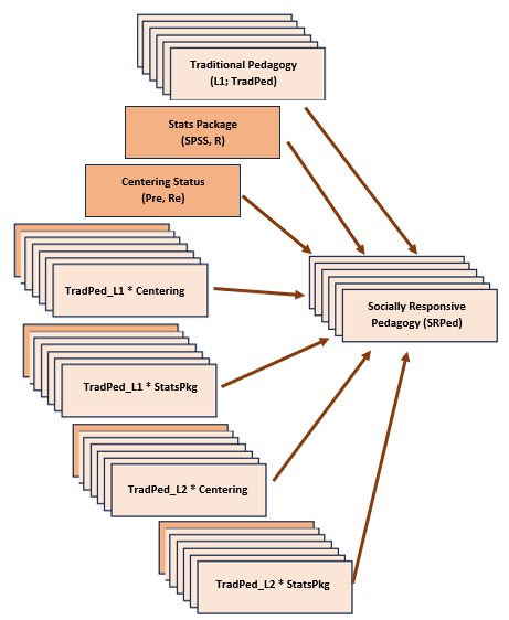
### Import the data and format the variables in the model
Scoring the variables.
TradPed_vars <- c("ClearResponsibilities", "EffectiveAnswers", "Feedback",
    "ClearOrganization", "ClearPresentation")
raw$TradPed <- sjstats::mean_n(raw[, ..TradPed_vars], 0.75)

SRPed_vars <- c("InclusvClassrm", "EquitableEval", "MultPerspectives",
    "DEIintegration")
raw$SRPed <- sjstats::mean_n(raw[, ..SRPed_vars], 0.75)

# If the scoring code above does not work for you, try the format
# below which involves inserting to periods in front of the variable
# list. One example is provided. raw$TradPed <- sjstats::mean_n(raw[,
# ..TradPed_vars], .75))
I will create a babydf to include only the variables in the analysis.
Restructure the dataset from wide to long (or from long to wide)
My data is long, so I will make it wide. I first need to give it an Index variable. In this data, students took ANOVA first, multivariate second, and psychometrics third.
longdf$Course <- factor(longdf$Course,levels = c("ANOVA", "Multivariate", "Psychometrics"))
str(longdf$Course)
## Factor w/ 3 levels "ANOVA","Multivariate",..: 1 1 1 1 1 1 1 1 1 1 ...longdf$Index <- plyr::mapvalues(longdf$Course, from = c('ANOVA', 'Multivariate', 'Psychometrics'), to = c(1, 2, 3))It seems like we can only do one L1 variable at a time.
library(data.table)
W1<-reshape2::dcast(longdf, deID + Centering ~ Index, value.var = c("Index"))
#rename the anxiety variable
W1<-  dplyr::rename(W1, Index1 = "1", Index2 = "2", Index3 = "3")
W2<-reshape2::dcast(longdf, deID ~ Index, value.var = c("TradPed"))
#rename the anxiety variable
W2<-  dplyr::rename(W2, TrP1 = "1", TrP2 = "2",TrP3 = "3")
#For remaining L1 variable, do them one at a time -- key them from the person-level ID and the wave/index.
W3<-reshape2::dcast(longdf, deID ~ Index, value.var = c("SRPed"))
W3<-  dplyr::rename(W3, SRP1 = "1", SRP2 = "2", SRP3 = "3")
#Next, join the dataframes by the person-level ID
#Only two can be joined at a time
widedf <- dplyr::full_join(W1, W2, by = c("deID"))
widedf <- dplyr::full_join(widedf, W3,  by = c("deID"))
13.9.1 Produce multilevel descriptive statistics and correlation matrix
##  Multilevel Descriptive Statistics
##
##                          TradPed  SRPed
##   Level 1
##    No. of cases              307    299
##    No. of missing values       3     11
##
##    Variance Within          0.27   0.16
##
##   Level 2
##    No. of clusters           141    140
##    Average cluster size     2.18   2.14
##    Min cluster size            1      1
##    Max cluster size            3      3
##
##    Mean                     4.23   4.52
##    Variance Between         0.34   0.19
##    ICC(1)                  0.555  0.545
##    ICC(2)                  0.732  0.724
##
##   Design effect             1.65   1.62
##   Design effect sqrt        1.29   1.27
##   Effective sample size   185.64 184.65
corrmatrix <- misty::multilevel.cor(longdf[, c("TradPed", "SRPed")], cluster = longdf$deID,
split = FALSE, output = TRUE, write = "MLMcorr.xlsx", print = c("cor",
"p"), digits = 3, missing = "listwise")## Within-Group and Between-Group Correlation Matrix
##
## lavaan 0.6.17
##
## Estimator ML
## Standard Errors Conventional
## Missing Data Listwise Deletion
##
## Used Total
## Number of Observations 298 310
## Number of Clusters 140
##
## TradPed SRPed
## TradPed 0.836
## SRPed 0.561
##
## Significance Value (p-value)
##
## TradPed SRPed
## TradPed 0.000
## SRPed 0.000
##
## Adjustment for multiple testing: none
##
## Note. n(within) = 298, n(between) = 140
## Lower triangular: Within-Group, Upper triangular: Between-Group## Within-Group and Between-Group Correlation Matrix
##
## lavaan 0.6.17
##
## Estimator ML
## Standard Errors Conventional
## Missing Data Listwise Deletion
##
## Used Total
## Number of Observations 298 310
## Number of Clusters 140
##
## TradPed SRPed
## TradPed 0.836
## SRPed 0.561
##
## Significance Value (p-value)
##
## TradPed SRPed
## TradPed 0.000
## SRPed 0.000
##
## Adjustment for multiple testing: none
##
## Note. n(within) = 298, n(between) = 140
## Lower triangular: Within-Group, Upper triangular: Between-GroupExplore data with an unfitted model
Quick way to obtain a random set from the long file.
## Classes 'data.table' and 'data.frame':   310 obs. of  6 variables:
##  $ deID     : int  1 2 3 4 5 6 7 8 9 10 ...
##  $ Course   : Factor w/ 3 levels "ANOVA","Multivariate",..: 1 1 1 1 1 1 1 1 1 1 ...
##  $ Centering: Factor w/ 2 levels "Pre","Re": 2 2 2 2 2 2 2 2 2 2 ...
##  $ TradPed  : num  4.4 3.8 4 3 4.8 3.5 4.6 3.8 3.6 4.6 ...
##  $ SRPed    : num  5 5 4.25 5 5 3.75 5 5 4.25 5 ...
##  $ Index    : Factor w/ 3 levels "1","2","3": 1 1 1 1 1 1 1 1 1 1 ...
##  - attr(*, ".internal.selfref")=<externalptr>
The exploratory plots I want to create require at least 3 pieces of data per person, so I will first create a sample of data where each person contributes 3 waves and data is non-missing. Please note – this is NOT the final set I will analyze. Rather, this will allow me a preview into the data to see if my “occular anlysis” (i.e., “just looking at it”) identifies any particular trends.
## ── Attaching core tidyverse packages ──────────────────────── tidyverse 2.0.0 ──
## ✔ forcats   1.0.0     ✔ stringr   1.5.1
## ✔ lubridate 1.9.2     ✔ tibble    3.2.1
## ✔ purrr     1.0.1     ✔ tidyr     1.3.0
## ✔ readr     2.1.4
## ── Conflicts ────────────────────────────────────────── tidyverse_conflicts() ──
## ✖ ggplot2::%+%()        masks psych::%+%()
## ✖ ggplot2::alpha()      masks psych::alpha(), scales::alpha()
## ✖ data.table::between() masks dplyr::between()
## ✖ readr::col_factor()   masks scales::col_factor()
## ✖ purrr::discard()      masks scales::discard()
## ✖ dplyr::filter()       masks stats::filter()
## ✖ data.table::first()   masks dplyr::first()
## ✖ lubridate::hour()     masks data.table::hour()
## ✖ lubridate::isoweek()  masks data.table::isoweek()
## ✖ dplyr::lag()          masks stats::lag()
## ✖ data.table::last()    masks dplyr::last()
## ✖ lubridate::mday()     masks data.table::mday()
## ✖ lubridate::minute()   masks data.table::minute()
## ✖ lubridate::month()    masks data.table::month()
## ✖ lubridate::quarter()  masks data.table::quarter()
## ✖ lubridate::second()   masks data.table::second()
## ✖ purrr::transpose()    masks data.table::transpose()
## ✖ lubridate::wday()     masks data.table::wday()
## ✖ lubridate::week()     masks data.table::week()
## ✖ lubridate::yday()     masks data.table::yday()
## ✖ lubridate::year()     masks data.table::year()
## ℹ Use the conflicted package (<http://conflicted.r-lib.org/>) to force all conflicts to become errorsFrom this complete set of data, I will creat a subsample of 30 sets of data.
#setting the random seed will mean that the same 30 are always pulled (even though the process is otherwise "random")
set.seed(20231113)

rndm30 <- subset(rndm30, deID %in% sample(unique(rndm30$deID), 30))## Factor w/ 3 levels "1","2","3": 3 3 3 3 3 3 3 3 3 3 ...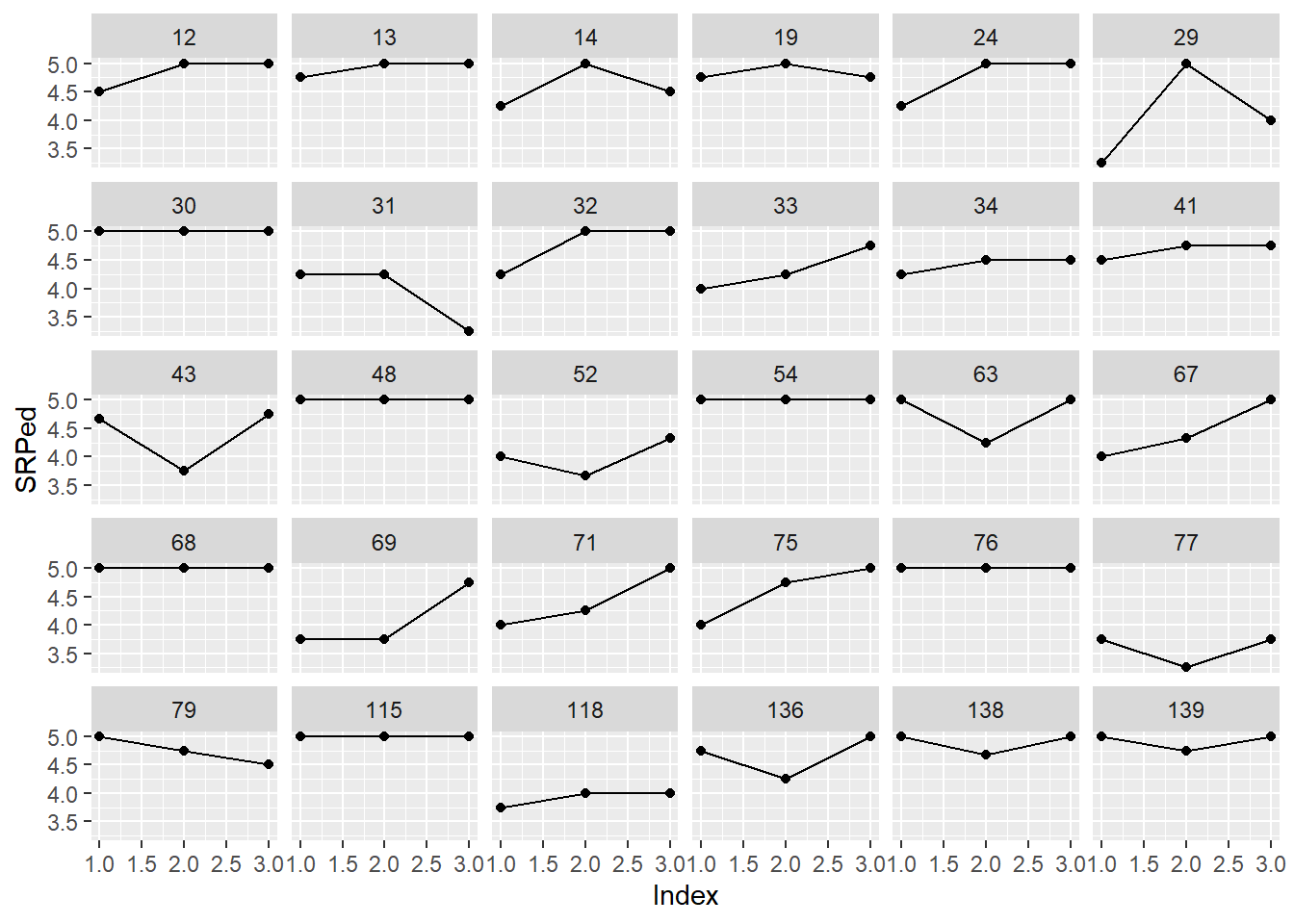
Explore data with a model fitted with a linear growth trajectory
ggplot(data = rndm30, aes(x = Index, y = SRPed)) + geom_point() + stat_smooth(method = "lm",
    se = FALSE) + facet_wrap(~deID)
## `geom_smooth()` using formula = 'y ~ x'
Explore data with the fitted (or unfitted) data identified by the L2 predictor
ggplot(data = rndm30, aes(x = Index, y = SRPed, linetype = Centering)) +
    geom_point() + geom_line() + facet_wrap(~deID)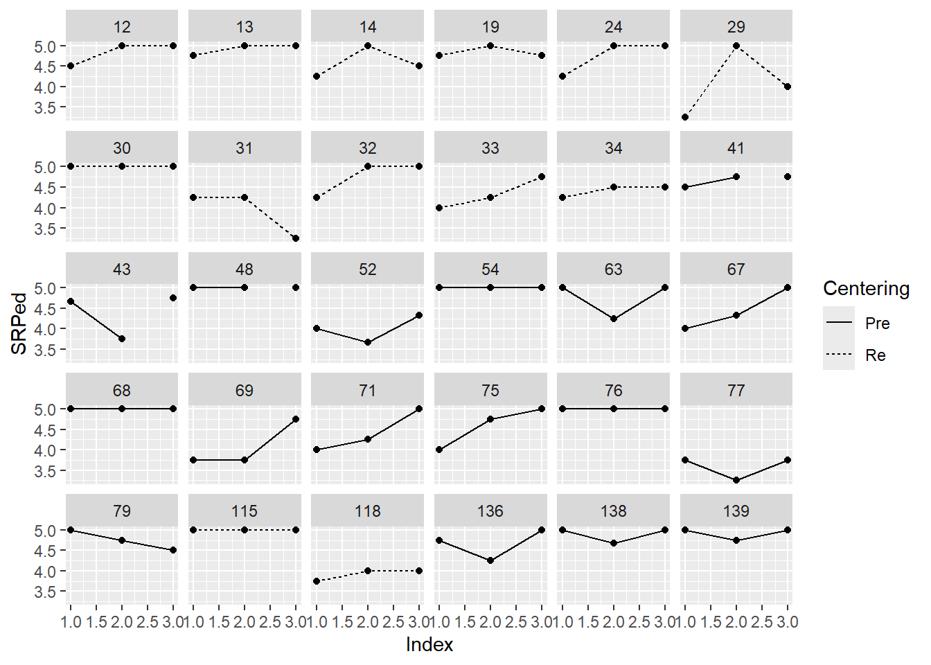
ggplot(data = rndm30, aes(x = Index, y = SRPed, linetype = Centering)) +
    geom_point() + stat_smooth(method = "lm", se = FALSE) + facet_wrap(~deID)
## `geom_smooth()` using formula = 'y ~ x'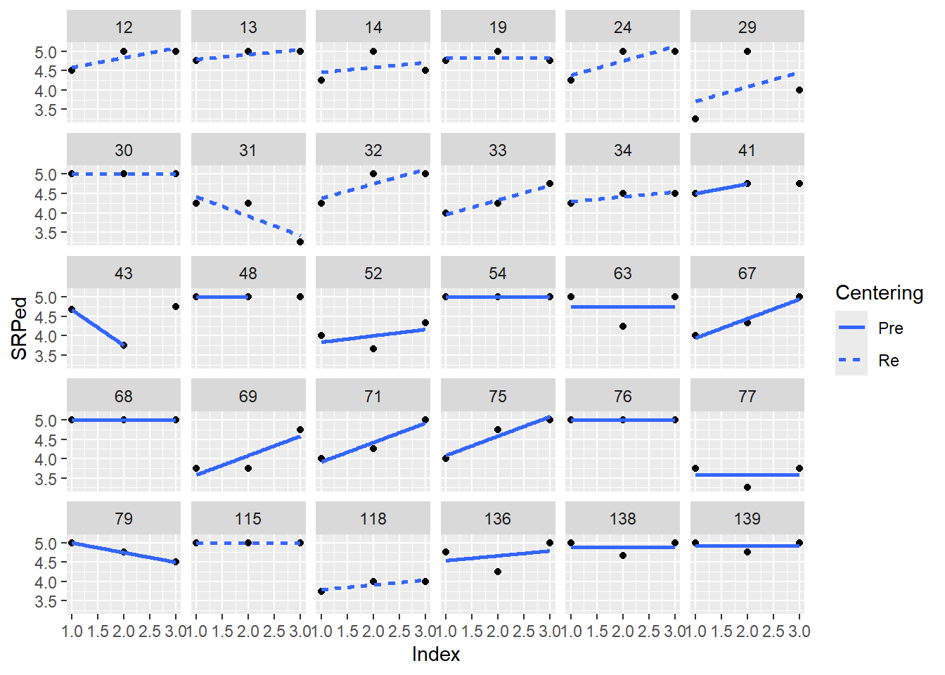
ggplot(data = rndm30) + geom_line(aes(x = Index, y = SRPed, color = as.factor(Centering), group = deID))