Chapter 1 Scrubbing
The focus of this chapter is the process of starting with raw data and preparing it for multivariate analysis. To that end, we will address the conceptual considerations and practical steps in “scrubbing and scoring.”
A twist in this lesson is that I am asking you to contribute to the dataset that serves as the basis for the chapter and the practice problems. In the spirit of open science, this dataset is available to you and others for your own learning. Before continuing, please take 15-20 minutes to complete the survey titled, Rate-a-Recent-Course: A ReCentering Psych Stats Exercise. The study is approved by the Institutional Review Board at Seattle Pacific University (SPUIRB# 202102011, no expiration). Details about the study, including an informed consent, are included at the link.
1.2 Workflow for Scrubbing
The same workflow guides us through the Scrubbing, Scoring, and Data Dx chapters. In this lesson we focus on downloading data from Qualtrics and determining which cases can be retained for analysis based on inclusion and exclusion criteria.
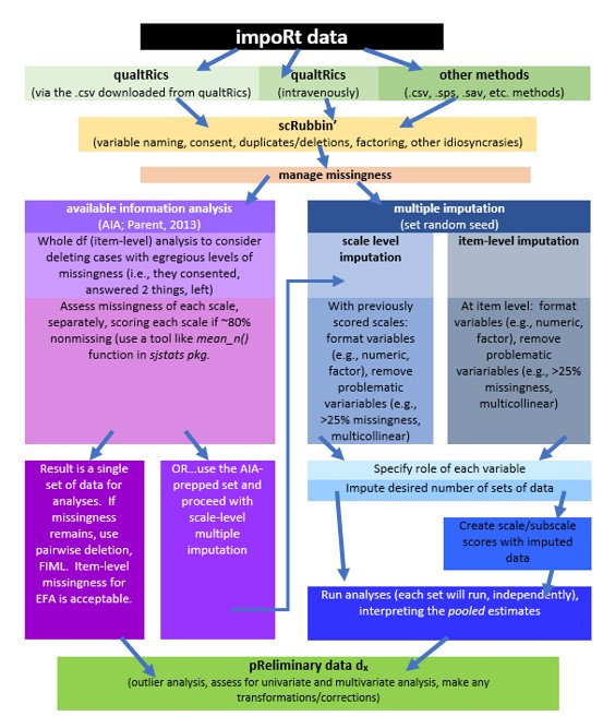
Here is a narration of the figure:
- The workflow begins by importing data into R. Most lessons in this series involve simulated data that are created directly in R. Alternatively, data could be:
- imported “intRavenously” through programs such as Qualtrics,
- exported from programs such as Qualtrics to another program (e.g., .xlxs, .csv),
- imported in other forms (e.g., .csv, .sps, .sav).
- Scrubbing data by
- variable naming,
- specifying variable characteristics such as factoring,
- ensuring that included participants consented to participation,
- determining and executing the inclusion and exclusion criteria.
- Conduct preliminary data diagnostics such as
- outlier analysis
- assessing for univariate and multivariate analysis
- making transformations and/or corrections
- Managing missingness by one of two routes
- Available information analysis (Parent, 2013) at either the item-level or scale level. The result is a single set of data for analysis. If missingness remains, options include pairwise deletion, listwise deletion, or specifying FIML (when available). Another option is to use multiple imputation.
- Multiple imputation at either scale level or item-level
1.3 Research Vignette
To provide first-hand experience as both the respondent and analyst for the same set of data, you were asked to complete a survey titled, Rate-a-Recent-Course: A ReCentering Psych Stats Exercise. If you haven’t yet completed it, please consider doing so, now. In order to reduce the potential threats to validity by providing background information about the survey, I will wait to describe it until later in the chapter.
The survey is administered in Qualtrics. In the chapter I teach two ways to import Qualtrics data into R. We will then use the data to work through the steps identified in the workflow.
1.4 Working the Problem
1.4.1 intRavenous Qualtrics
I will demonstrate using a Qualtrics account at my institution, Seattle Pacific University. The only surveys in this account are for the Recentering Psych Stats chapters and lessons. The surveys were designed to not capture personally identifying information.
Access credentials for the institutional account, individual user’s account, and survey are essential for getting the survey items and/or results to export into R. The Qualtrics website provides a tutorial for generating an API token.
We need two pieces of information: the root_url and an API token. To retrieve these:
- Log into your respective qualtrics.com account
- Select Account Settings
- Choose “Qualtrics IDs” from the user name dropdown
The root_url is the first part of the web address for the Qualtrics account. For our institution it is: spupsych.az1.qualtrics.com .
The API token is in the box labeled, “API.” If it is empty, select, “Generate Token.” If you do not have this option, locate the brand administrator for your Qualtrics account. They will need to set up your account so that you have API privileges.
BE CAREFUL WITH THE API TOKEN This is the key to your Qualtrics accounts. If you leave it in an .rmd file that you forward to someone else or upload to a data repository, this key and the base URL gives access to every survey in your account. If you share it, you could be releasing survey data to others that would violate confidentiality promises in an IRB application.
If you mistakenly give out your API token you can generate a new one within your Qualtrics account and re-protect all its contents.
You do need to change the API key/token if you want to download data from a different Qualtrics account. If your list of surveys generates the wrong set of surveys, restart R, make sure you have the correct API token and try again.
# You only need to run this ONCE to draw from the same Qualtrics
# account. If you change Qualtrics accounts you will need to get a
# different token.

# qualtRics::qualtrics_api_credentials(api_key =
# 'mUgPMySYkiWpMFkwHale1QE5HNmh5LRUaA8d9PDg', base_url =
# 'spupsych.az1.qualtrics.com', overwrite = TRUE, install = TRUE)

# readRenviron('~/.Renviron')
all_surveys() generates a dataframe containing information about all the surveys stored on your Qualtrics account.
# surveys <- qualtRics::all_surveys()

# View this as an object (found in the right: Environment).  Get
# survey id # for the next command If this is showing you the WRONG
# list of surveys, you are pulling from the wrong Qualtrics account
# (i.e., maybe this one instead of your own). Go back and change your
# API token (it saves your old one). Changing the API likely requires
# a restart of R.
To retrieve the survey, use the fetch_survey() function.
# obtained with the survey ID
#'surveyID' should be the ID from above
#'verbose' prints messages to the R console
#'label', when TRUE, imports data as text responses; if FALSE prints the data as numerical responses
#'convert', when TRUE, attempts to convert certain question types to the 'proper' data type in R; because I don't like guessing, I want to set up my own factors.
#'force_request', when TRUE, always downloads the survey from the API instead of from a temporary directory (i.e., it always goes to the primary source)
# 'import_id', when TRUE includes the unique Qualtrics-assigned ID;
# since I have provided labels, I want false

# QTRX_df <-qualtRics::fetch_survey(surveyID = 'SV_b2cClqAlLGQ6nLU',
# time_zone = NULL, verbose = FALSE, label=FALSE, convert=FALSE,
# force_request = TRUE, import_id = FALSE)

# useLocalTime = TRUE,
It is possible to import Qualtrics data that has been downloaded from Qualtrics as a .csv. I demo this in the Bonus Reel at the end of this lesson.
In prior versions of this chapter I allowed the chapter to automatically update with “all the new data” each time the OER was re-rendered/built. Because I think this caused confusion, I have decided to save the data in both .csv and .rds versions, then clear my environment, upload the .rds (my personal favorite format) version, and demonstrate the scrubbing techniques with that data. If you continue with data you just downloaded from Qualtrics, you will get different answers than are in the lesson. While I think that continuing with the most current data set is a viable option for a practice problem, it could be confusing. Rather, follow one of the two options below to upload .csv or .rds versions of the data I used in the lesson.
1.4.1.1 Option 1. Upload an .rds file
Because .rds files will retain any formatting information we provide about variables, I like using them. The downside is that you cannot simply open and view them outside of the R environment. Here is the code I used to produce the .rds version of the file. If you want to obtain the same results as I report in the chapter, do NOT run it again.
# to save the df as an .rds (think 'R object') file on your computer;
# it should save in the same file as the .rmd file you are working
# with saveRDS(QTRX_df, 'QTRX_df230902.rds')
Rather, head to the MultivModel GitHub site and download the QTRX_df230902b.rds file. Place it in the same folder as the .rmd you are using and run the code below. And actually, I further re-named the file that you will retrieve so that it won’t be over-written.*
Occasionally, I have had a student for whom the .rds files don’t seem to work. Uploading a .csv file is an option.
1.4.1.2 Option 2. Upload a .csv file
Simply for your information, here is the code I used to produce the .csv version of the file. If you want to obtain the same results as I report in the chapter, do NOT run it again.
# write the simulated data as a .csv write.table(QTRX_df,
# file='QTRX_df230902.csv', sep=',', col.names=TRUE, row.names=FALSE)
Rather, head to the MultivModel GitHub site and download the QTRX_df230902b.csv file. Place it in the same folder as the .rmd you are using and run the code below. And actually, I further re-named the file that you will retrieve so that it won’t be over-written.
# bring back the simulated dat from a .csv file QTRX_df <-
# read.csv('QTRX_df230902b.csv', header = TRUE)
You need not do both. That is, either download-and-import either the .rds or .csv file.
1.4.2 About the Rate-a-Recent-Course Survey
As a teaching activity for the ReCentering Psych Stats OER, the topic of the survey was selected to be consistent with the overall theme of OER. Specifically, the purpose of this study is to understand the campus climate for students whose identities make them vulnerable to bias and discrimination. These include students who are Black, non-Black students of color, LGBTQ+ students, international students, and students with disabilities.
Although the dataset should provide the opportunity to test a number of statistical models, one working hypothesis that framed the study is that the there will be a greater sense of belonging and less bias and discrimination when there is similar representation (of identities that are often marginalized) in the instructional faculty and student body. Termed, “structural diversity” (K. R. Lewis & Shah, 2019) this is likely an oversimplification. In fact, an increase in diverse representation without attention to interacting factors can increase hostility on campus (Hurtado, 2007). Thus, we included the task of rating of a single course relates to the larger campus along the dimensions of belonging and bias/discrimination. For example, if a single class has higher ratings on issues of inclusivity, diversity, and respect, we would expect that sentiment to be echoed in the broader institution.
Our design has notable limitations You will likely notice that we ask about demographic characteristics of the instructional staff and classmates in the course rated, but we do not ask about the demographic characteristics of the respondent. In making this decision, we likely lose important information; Iacovino and James (2016) have noted that White students perceive campus more favorably than Black student counterparts. We made this decision to protect the identity of the respondent. As you will see when we download the data, if a faculty member asked an entire class to take the survey, the datestamp and a handful of demographic identifiers could very likely identify a student. In certain circumstances, this might be risky in that private information (i.e., gender nonconformity, disclosure of a disability) or course evaluation data could be related back to the student.
Further, the items that ask respondents to guess the identities of the instructional staff and classmates are limited, and contrary to best practices in survey construction that recommend providing the option of a “write-in” a response. After consulting with a diverse group of stakeholders and subject matter experts (and revising the response options numerous times) I have attempted to center anti-Black racism in the U.S. (Mosley et al., 2020, 2021; Singh, 2020). In fact, the display logic does not present the race items when the course is offered outside the U.S. There are only five options for race: biracial/multiracial, Black, non-Black person(s) of color, White, and I did not notice (intended to capture a color-blind response). One unintended negative consequence of this design is that the response options could contribute to colorism (Adames et al., 2021; Capielo Rosario et al., 2019). Another possibility is that the limited options may erase, or make invisible, other identities. At the time that I am writing the first draft of this chapter, the murder of six Asian American women in Atlanta has just occurred. The Center for the Study of Hate and Extremeism has documented that while overall hate crimes dropped by 7% in 2020, anti-Asian hate crimes reported to the police in America’s largest cities increasedby 149% (FACT SHEET, n.d.). These incidents have occurred not only in cities, but in our neighborhoods and on our campusus (P. Kim, 2021; Paul Y. Kim, 2021; STOP AAPI HATE, n.d.). While this survey is intended to assess campus climate as a function of race, it unfortunately does not distinguish between many identities that experience marginalization.
In parallel, the items asking respondents to identity characteristics of the instructional staff along dimensions of gender, international status, and disability are “large buckets” and do not include “write-in” options. Similarly, there was no intent to cause harm by erasing or making invisible individuals whose identities are better defined by different descriptors. Further, no write-in items were allowed. This was also intentional to prevent potential harm caused by people who could leave inappropriate or harmful comments.
1.4.3 The Codebook
In order to scrub-and-score a survey, it is critical to know about its content, scoring directions for scales/subscales, and its design. A more complete description of the survey design elements is (or will be) available in the Recentering Psych Stats: Psychometric OER. The review in this chapter provides just-enough information to allow us to make decisions about which items to retain and how to score them. When they are well-written, information in the IRB application and pre-registration can be helpful in the scrubbing and scoring process.
Let’s look “live” at the survey. In Qualtrics it is possible to print a PDF that looks very similar to its presentation when someone is taking it. You can access that static version here.
We can export a codebook, that is, a Word (or PDF) version of the survey with all the coding. In Qualtrics the protocol is: Survey/Tools/ImportExport/Export Survey to Word. Then select all the options you want (especially “Show Coded Values”). A tutorial provided by Qualtrics can be found here. This same process can be used to print the PDF example I used above.
It is almost impossible to give this lecture without some reference to Qualtrics and the features used in Qualtrics. An import of raw data from Qualtrics into R can be nightmare in that the Qualtrics-assigned variable names are numbers (e.g., QID1, QID2) – but often out of order because the number is assigned when the question is first created. If the survey is reordered, the numbers get out of sequence.
Similarly, values for Likert-type scales can also get out of order if the scale anchors are revised (which is common to do).
I recommend providing custom variable names and recode values directly in Qualtrics before exporting them into R. A Qualtrics tutorial for this is provided here. In general, consider these qualities when creating variable names:
- Brevity: historically, SPSS variable names could be a maximum of 8 characters.
- Intuitive: although variables can be renamed in R (e.g., for use in charts and tables), it is helpful when the name imported from Qualtrics provides some indication of what the variable is.
- Systematic: start items in a scale with the same stem, followed by the item number – ITEM1, ITEM2, ITEM3.
The Rate-a-Recent-Course survey was written using some special features in Qualtrics. These include
- Display logic
- Items that are U.S.-centric are only shown if the respondent is taking a course from an institution in the U.S. is a student in the U.S.
- Loop and merge
- Because course may have multiple instructional staff, the information asking about demographic characteristics of the instructors is repeated according to the number input by the respondent
- Random presentation of the 30 items asking about campus climate for the five groups of students
- Although this might increase the cognitive load of the survey, this helps “spread out” missingness for respondents who might tire of the survey and stop early
- Rank ordering of the institutional level (department, school/faculty, campus/university) to which the respondent feels most connected
Looking at the QTRX_df, StartDate thru UserLanguage are metadata created by Qualtrics. The remaining variables and associated value labels are in the codebook.
1.5 Scrubbing
With a look at our survey, codebook, and imported data, we now get to the business of scRubbing (deleting those who did not give consent, deleting previews, etc.). This level of “scrubbing” precedes the more formal detection of outliers.
1.5.1 Tools for Data Manipulation
The next stages will provide some experience manipulating data with dplyr from the tidyverse.
The tidyverse is a system of packages (i.e,. when you download the tidyverse, you download all its packages/members) for data manipulation, exploration and visualization. The packages in the tidyverse share a common design philosophy. These were mostly developed by Hadley Wickham, but more recently, more designers are contributing to them. Tidyverse packages are intended to make statisticians and data scientists more productive by guiding them through workflows that facilitate communication and result in reproducible work products. Fundamentally, the tidyverse is about the connections between the tools that make the workflow possible. Critical packages in the tidyverse include:
- dplyr: data manipulation: mutate, select, filter, summarize, arrange
- ggplot2: extravagant graphing
- tibble: a tibble is a dataframe that provides the user with more (and less) control over the data.
- readr: gives access to “rectangular data” like .csv and tables
- tidyr: tidy data is where each variable is a column, each observation is a row, each value is a cell (duh). tidyr’s contributions are gather(wide to long) and spread(long to wide) as well as separate, extract, unite.
- purrr: facilitates working with functions and vectors. For example, if you write a function, using purrr may help you replace loops with code that is more efficient and intuitive.
The tidyverse is ever-evolving – so check frequently for updates and troubleshooting.
A handy cheatsheet for data transformation is found here.
1.5.2 Inclusion and Exclusion Criteria
For me, the first pass at scrubbing is to eliminate the obvious. In our case this is includes previews and respondents who did not consent to continue. Previews are the researcher-initiated responses usually designed to proofread or troubleshoot survey problems. There could be other first-pass-deletions, such as selecting response between certain dates.
I think these first-pass deletions, especially the ones around consent, are important to do as soon as possible. Otherwise, we might delete some of the variables (e.g., timestamps, consent documentation, preview status) and neglect to delete these cases later in the process.
We are here in the workflow:
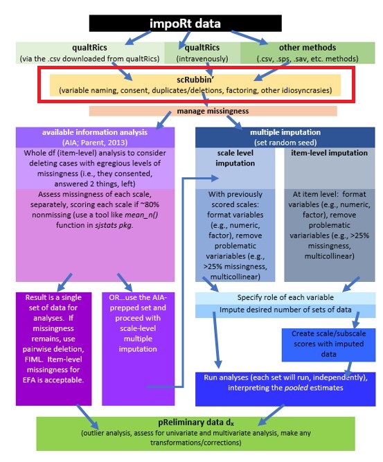
We can either update the existing df (by using the same object), or creating a new df from the old. Either works. In my early years, I tended to create lots of new objects. As I have gained confidence in myself and in R, I’m inclined to update the existing df. Why? Because unless you write the object as an outfile (using the same name for the object as for the filename – which I do not recommend), the object used in R does not change the source of the dat. Therefore, it is easy to correct early code and it keeps the global environment less cluttered.
In this particular survey, the majority of respondents will take the survey because they clicked an anonymous link provided by Qualtrics. Another Qualtrics distribution method is e-mail. At the time of this writing, we have not recruited by e-mail, but it is is possible we could do so in the future. What we should not include, though, are previews. These are the times when the researcher is self-piloting the survey to look for errors and to troubleshoot.
# the filter command is used when we are making inclusion/exclusion
# decisions about rows != means do not include cases with 'preview'

QTRX_df <- dplyr::filter(QTRX_df, DistributionChannel != "preview")

# FYI, another way that doesn't use tidyverse, but gets the same
# result QTRX_df <- QTRX_df[!QTRX_df$DistributionChannel ==
# 'preview',]
APA Style, and in particular the Journal Article Reporting Standards (JARS) for quantitative research specify that we should report the frequency or percentages of missing data. We would start our counting after eliminating the previews.
# I created an object that lists how many rows/cases remain.  I used
# inline text below to update the text with the new number
nrow(QTRX_df)
[1] 107CAPTURING RESULTS FOR WRITING IT UP:
Data screening suggested that 107 individuals opened the survey link.
Next let’s filter in only those who consented to take the survey. Because Qualtrics discontinued the survey for everyone who did not consent, we do not have to worry that their data is unintentionally included, but it can be useful to mention the number of non-consenters in the summary of missing data.
[1] 83CAPTURING RESULTS FOR WRITING IT UP:
Data screening suggested that 107 individuals opened the survey link. Of those, 83 granted consent and proceeded into the survey items.
In this particular study, the categories used to collect informtaion about race/ethnicity were U.S.-centric. Thus, they were only shown if the respondent indicated that the course being rated was taught by an institution in the U.S. Therefore, an an additional inclusion criteria for this specific research model should be that the course was taught in the U.S.
[1] 69CAPTURING RESULTS FOR WRITING IT UP:
Data screening suggested that 107 individuals opened the survey link. Of those, 83 granted consent and proceeded into the survey items. A further inclusion criteria was that the course was taught in the U.S; 69 met this criteria.
1.5.3 Renaming Variables
Even though we renamed the variables in Qualtrics, the loop-and-merge variables were auto-renamed such that they each started with a number. I cannot see how to rename these from inside Qualtrics. A potential problem is that, in R, when variable names start with numbers, they need to be surrounded with single quotation marks. I find it easier to rename them now. I used “i” to start the variable name to represent “instructor.”
The form of the rename() function is this: df_named <- rename(df_raw, NewName1 = OldName1)
QTRX_df <- dplyr::rename(QTRX_df, iRace1 = "1_iRace", iRace2 = "2_iRace",
    iRace3 = "3_iRace", iRace4 = "4_iRace", iRace5 = "5_iRace", iRace6 = "6_iRace",
    iRace7 = "7_iRace", iRace8 = "8_iRace", iRace9 = "9_iRace", iRace10 = "10_iRace")
Also in Qualtrics, it was not possible to rename the variable (formatted with sliders) that asked respondents to estimate the proportion of classmates in each race-based category. Using the codebook, we can do this now. I will use “cm” to precede each variable name to represent “classmates.”
QTRX_df <- dplyr::rename(QTRX_df, cmBiMulti = Race_10, cmBlack = Race_1,
    cmNBPoC = Race_7, cmWhite = Race_8, cmUnsure = Race_2)
Let’s also create an ID variable (different from the lengthy Qualtrics-issued ID) and then move it to the front of the distribution.
── Attaching core tidyverse packages ──────────────────────── tidyverse 2.0.0 ──
✔ dplyr     1.1.2     ✔ readr     2.1.4
✔ forcats   1.0.0     ✔ stringr   1.5.1
✔ ggplot2   3.5.0     ✔ tibble    3.2.1
✔ lubridate 1.9.2     ✔ tidyr     1.3.0
✔ purrr     1.0.1
── Conflicts ────────────────────────────────────────── tidyverse_conflicts() ──
✖ dplyr::filter() masks stats::filter()
✖ dplyr::lag()    masks stats::lag()
ℹ Use the conflicted package (<http://conflicted.r-lib.org/>) to force all conflicts to become errors1.5.4 Downsizing the Dataframe
Although researchers may differ in their approach, my tendency is to downsize the df to the variables I will be using in my study. These could include variables in the model, demographic variables, and potentially auxiliary variables (i.e,. variables not in the model, but that might be used in the case of multiple imputation).
This particular survey did not collect demographic information, so that will not be used. The model that I will demonstrate in this research vignette examines the the respondent’s perceived campus climate for students who are Black, predicted by the the respondent’s own campus belonging, and also the structural diversity (K. R. Lewis & Shah, 2019) proportions of Black students in the classroom and BIPOC (Black, Indigenous, and people of color) instructional staff.
I would like to assess the model by having the instructional staff variable to be the %Black instructional staff. At the time that this lecture is being prepared, there is not sufficient Black representation in the staff to model this.
The select() function can let us list the variables we want to retain.
# You can use the ':' to include all variables from the first to last
# variable in any sequence; I could have written this more
# efficiently.  I just like to 'see' my scales and clusters of
# variables.

Model_df <- (dplyr::select(QTRX_df, ID, iRace1, iRace2, iRace3, iRace4,
    iRace5, iRace6, iRace7, iRace8, iRace9, iRace10, cmBiMulti, cmBlack,
    cmNBPoC, cmWhite, cmUnsure, Belong_1:Belong_3, Blst_1:Blst_6))
It can be helpful to save outfile of progress as we go along. Here I save this raw file. I will demonstrate how to save both .rds and .csv files.
1.6 Toward the APA Style Write-up
Because we have been capturing the results as we have worked the problem, our results section is easy to assemble.
1.7 Practice Problems
Starting with this chapter, the practice problems for this and the next two chapters (i.e., Scoring, Data Dx) are intended to be completed in a sequence. Whatever practice option(s) you choose, please
- Use raw data that has some missingness (as a last resort you could manually delete some cells),
- Includes at least 3 independent/predictor variables
- these could be categorically or continuously scaled
- at least one variable should require scoring.
- Include at least 1 dependent variable
- at this point in your learning it should be continuously scaled
The three problems below are listed in the order of graded complexity. If you are just getting started, you may wish to start with the first problem. If you are more confident, choose the second or third option. You will likely encounter challenges that were not covered in this chapter. Search for and try out solutions, knowing that there are multiple paths through the analysis.
1.7.1 Problem #1: Rework the Chapter Problem
Because the Rate-a-Recent-Course survey remains open, it is quite likely that there will be more participants who have taken the survey since this chapter was last updated. If not – please encourage a peer to take it. Even one additional response will change the results. This practice problem encourages you to rework the chapter, as written, with the updated data from the survey.
1.7.2 Problem #2: Use the Rate-a-Recent-Course Survey, Choosing Different Variables
Before starting this option, choose a minimum of three variables from the Rate-a-Recent-Course survey to include in a simple statistical model. Work through the chapter making decisions that are consistent with the research model you have proposed. There will likely be differences at several points in the process. For example, you may wish to include (not exclude) data where the rated-course was offered by an institution outside the U.S. Different decisions may involve an internet search for the R script you will need as you decide on inclusion and exclusion criteria.
1.7.3 Problem #3: Other data
Using raw data for which you have access, use the chapter as a rough guide. Your data will likely have unique characteristics that may involved searching for solutions beyond this chapter/OER.
1.7.4 Grading Rubric
Regardless which option(s) you chose, use the elements in the grading rubric to guide you through the practice.
| Assignment Component | Points Possible | Points Earned |
|---|---|---|
| 1. Specify a research model that includes three predictor variables (continuously or categorically scaled) and one dependent (continuously scaled) variable | 5 | _____ |
| 2. Import data | 5 | _____ |
| 3. Include only those who consented\(^*\) | 5 | _____ |
| 4. Apply exclusionary criteria \(^*\) | 5 | _____ |
| 5. Rename variables to be sensible and systematic \(^*\) | 5 | _____ |
| 6. Downsize the dataframe to the variables of interest | 5 | _____ |
| 7. Provide an APA style write-up of these preliminary steps | 5 | _____ |
| 8. Explanation to grader | 5 | _____ |
| Totals | 40 | _____ |
\(^*\) If your dataset does not require these steps, please provide example code that uses variables in your dataset. For example, for the inclusion or exclusion criteria, provide an example of how to filter in (or out) any variable on the basis of one of the response options. Once demonstrated, hashtag it out and rerun your script with those commands excluded.
A homeworked example for the Scrubbing, Scoring, and DataDx lessons (combined) follows the Data Dx lesson.
1.8 Bonus Track:

1.8.1 Importing data from an exported Qualtrics .csv file
The lecture focused on the “intRavenous” import. It is is also possible to download the Qualtrics data in a variety of formats (e.g., CSV, Excel, SPSS). Since I got started using files with the CSV extension (think “Excel” lite), that is my preference.
In Qualtrics, these are the steps to download the data: Projects/YOURsurvey/Data & Analysis/Export & Import/Export data/CSV/Use numeric values
I think that it is critical that to save this file in the same folder as the .rmd file that you will use with the data.
R is sensitive to characters used filenames As downloaded, my Qualtrics .csv file had a long name with spaces and symbols that are not allowed. Therore, I gave it a simple, sensible, filename, “ReC_Download210319.csv”. An idiosyncracy of mine is to datestamp filenames. I use two-digit representations of the year, month, and date so that if the letters preceding the date are the same, the files would alphabetize automatically.
library(qualtRics)
QTRX_csv <- read_survey("ReC_Download210319.csv", strip_html = TRUE, import_id = FALSE,
    time_zone = NULL, legacy = FALSE)
── Column specification ────────────────────────────────────────────────────────
cols(
  .default = col_double(),
  StartDate = col_datetime(format = ""),
  EndDate = col_datetime(format = ""),
  RecordedDate = col_datetime(format = ""),
  ResponseId = col_character(),
  DistributionChannel = col_character(),
  UserLanguage = col_character(),
  Virtual = col_number(),
  `5_iPronouns` = col_logical(),
  `5_iGenderConf` = col_logical(),
  `5_iRace` = col_logical(),
  `5_iUS` = col_logical(),
  `5_iDis` = col_logical(),
  `6_iPronouns` = col_logical(),
  `6_iGenderConf` = col_logical(),
  `6_iRace` = col_logical(),
  `6_iUS` = col_logical(),
  `6_iDis` = col_logical(),
  `7_iPronouns` = col_logical(),
  `7_iGenderConf` = col_logical(),
  `7_iRace` = col_logical()
  # ... with 17 more columns
)
ℹ Use `spec()` for the full column specifications.
Although minor tweaking may be required, the same script above should be applicable to this version of the data.