Chapter 9 One-Way Repeated Measures ANOVA
In the prior lessons, a critical assumption is that the observations must be “independent.” That is, related people (partners, parent/child, manager/employee) cannot comprise the data and there cannot be multiple waves of data for the same person. Repeated measures ANOVA is created specifically for this dependent purpose. This lessons focuses on the one-way repeated measures ANOVA, where we measure changes across time.
9.2 Introducing One-way Repeated Measures ANOVA
There are a couple of typical use cases for one-way repeated measures ANOVA. In the first, the research participant is assessed in multiple conditions – with no interested in change-over-time.
An example of a research design using this approach occurred in the Green and Salkind (2017b) statistics text, the one-way repeated measures vignette compared teachers’ perception of stress when responding to parents, teachers, and school administrators.

Another common use case is about time. The classic design is a pre-test, an intervention, a post-test, and a follow up. In designs like these researchers often hope that there is a positive change from pre-to-post and that that change either stays constant (from post-to-follow-up) or, perhaps, increases even further. The research vignette for this lesson is interested in change-over-time.

9.2.1 Workflow for Oneway Repeated Measures ANOVA
The following is a proposed workflow for conducting a one-way repeated measures ANOVA.
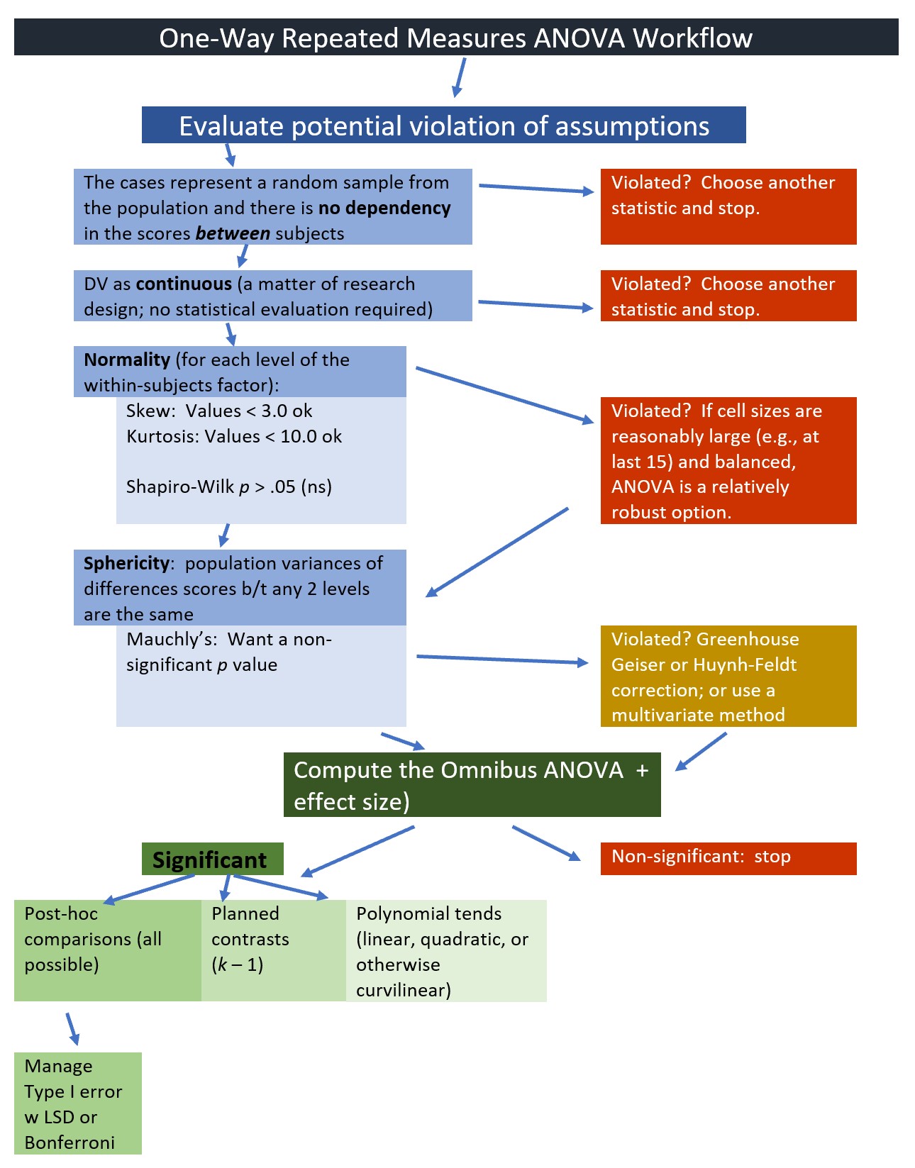
Steps involved in analyzing the data include:
- Preparing and importing the data.
- Exploring the data
- graphs
- descriptive statistics
- Checking distributional assumptions
- assessing normality via skew, kurtosis, Shapiro Wilks
- checking or violation of the sphericity assumption with Mauchly’s test; if violated interpret the corrected output or use a multivariate approach for the analysis
- Computing the omnibus ANOVA
- Computing post hoc comparisons, planned contrasts, or polynomial trends
- Managing Type I error
- Sample size/power analysis (which you should think about first – but in the context of teaching ANOVA, it’s more pedagogically sensible, here)
9.3 Research Vignette
Amodeo (Amodeo et al., 2018) and colleagues conducted a mixed methods study (qualitative and quantitative) to evaluate the effectiveness of an empowerment, peer-group-based, intervention with participants (N = 8) who experienced transphobic episodes. Focus groups used qualitative methods to summarize emergent themes from the program (identity affirmation, self-acceptance, group as support) and a one-way, repeated measures ANOVA provided evidence of increased resilience from pre to three-month followup.
Eight participants (seven transgender women and one genderqueer person) participated in the intervention. The mean age was 28.5 (SD = 5.85). All participants were located in Italy.
The within-subjects condition was wave, represented by T1, T2, and T3:
- T1, beginning of training
- Training, three 8-hour days,
- content included identity and heterosexism, sociopolitical issues and minority stress, resilience, and empowerment
- T2, at the conclusion of the 3-day training
- Follow-up session 3 months later
- T3, at the conclusion of the +3 month follow-up session
The dependent variable (assessed at each wave) was a 14-item resilience scale (Wagnild & Young, 1993). Items were assessed on a 7-point scale ranging from strongly disagree to strongly agree with higher scores indicating higher levels of resilience. An example items was, “I usually manage one way or another.”

9.3.1 Data Simulation
Below is the code I used to simulate data. The following code assumes 8 participants who each participated in 3 waves (pre, post, followup).
set.seed(2022)
#gives me 8 numbers, assigning each number 3 consecutive spots, in sequence
ID<-factor(c(rep(seq(1,8),each=3)))
#gives me a column of 24 numbers with the specified Ms and SD
Resilience<-rnorm(24,mean=c(5.7,6.21,6.26),sd=c(.88,.79,.37))
#repeats pre, post, follow-up once each, 8 times
Wave<-rep(c("Pre","Post", "FollowUp"),each=1,8)
Amodeo_long<-data.frame(ID, Wave, Resilience)
Let’s take a look at the structure of our variables. We want ID to be a factor, Resilience to be numeric, and Wave to be an ordered factor (Pre, Post, FollowUp).
'data.frame':   24 obs. of  3 variables:
 $ ID        : Factor w/ 8 levels "1","2","3","4",..: 1 1 1 2 2 2 3 3 3 4 ...
 $ Wave      : chr  "Pre" "Post" "FollowUp" "Pre" ...
 $ Resilience: num  6.49 5.28 5.93 4.43 5.95 ...
We need to update Wave to be an ordered factor. Because R’s default is to order factors alphabetically, we can use the levels command and identify our preferred order.
We check the structure again.
'data.frame':   24 obs. of  3 variables:
 $ ID        : Factor w/ 8 levels "1","2","3","4",..: 1 1 1 2 2 2 3 3 3 4 ...
 $ Wave      : Factor w/ 3 levels "Pre","Post","FollowUp": 1 2 3 1 2 3 1 2 3 1 ...
 $ Resilience: num  6.49 5.28 5.93 4.43 5.95 ...
9.3.1.0.1 Shape Shifters
The form of our data matters. The simulation created a long form (formally called the person-period form) of data. That is, each observation for each person is listed in its own row. In this dataset where we have 8 people with 3 observation (pre, post, follow-up) each, we have 24 rows. This is convenient, because this is the form we need for repeated measures ANOVA.
However, for some of the calculations (particularly those we will do by hand), we need the data to be in its more familiar wide form (formally called the person level form). We can do this with the data.table and reshape2()* packages.
# Create a new df (Amodeo_wide)
# Identify the original df
# We are telling it to connect the values of the Resilience variable its respective Wave designation
Amodeo_wide <- reshape2::dcast(data = Amodeo_long, formula =ID~Wave, value.var = "Resilience")
#doublecheck to see if they did what you think
str(Amodeo_wide)
'data.frame': 8 obs. of 4 variables:
$ ID : Factor w/ 8 levels "1","2","3","4",..: 1 2 3 4 5 6 7 8
$ Pre : num 6.49 4.43 4.77 5.91 4.84 ...
$ Post : num 5.28 5.95 6.43 7 6.28 ...
$ FollowUp: num 5.93 5.19 6.54 6.19 6.24 ...In this reshape script, I asked for a quick structure check. The format of the variables looks correct.
If you want to export these data as files to your computer, remove the hashtags to save (and re-import) them as .rds (R object) or .csv (“Excel lite”) files. This is not a necessary step to continue working the problem in this lesson.
The code for the .rds file will retain the formatting of the variables, but is not easy to view outside of R. I would choose this option.
#to save the df as an .rds (think "R object") file on your computer;
#it should save in the same file as the .rmd file you are working with
#saveRDS(Amodeo_long, "Amodeo_longRDS.rds")
#saveRDS(Amodeo_wide, "Amodeo_wideRDS.rds")
#bring back the simulated dat from an .rds file
#Amodeo_long <- readRDS("Amodeo_longRDS.rds")
#Amodeo_wide <- readRDS("Amodeo_wideRDS.rds")
Another option is to write them as .csv files. The code for .csv will likely lose any variable formatting, but the .csv file is easy to view and manipulate in Excel. If you choose this option, you will probably need to re-run the prior code to reformat Wave as an ordered factor
#write the simulated data as a .csv
#write.table(Amodeo_long, file="Amodeo_longCSV.csv", sep=",", col.names=TRUE, row.names=FALSE)
#write.table(Amodeo_wide, file="Amodeo_wideCSV.csv", sep=",", col.names=TRUE, row.names=FALSE)
#bring back the simulated dat from a .csv file
#Amodeo_long <- read.csv ("Amodeo_longCSV.csv", header = TRUE)
#Amodeo_wide <- read.csv ("Amodeo_wideCSV.csv", header = TRUE)
9.3.2 Quick peek at the data
Before we get into the statistic let’s inspect our data. As we work the problem we will switch between long and wide formats. We can start with the long form.
'data.frame':   24 obs. of  3 variables:
 $ ID        : Factor w/ 8 levels "1","2","3","4",..: 1 1 1 2 2 2 3 3 3 4 ...
 $ Wave      : Factor w/ 3 levels "Pre","Post","FollowUp": 1 2 3 1 2 3 1 2 3 1 ...
 $ Resilience: num  6.49 5.28 5.93 4.43 5.95 ...
In the following output, note the order of presentation of the grouping variable (i.e., FollowUp, Post, Pre). Even though we have ordered our factor so that “Pre” is first, the describeBy() function seems to be ordering them alphabetically.
    item   group1 vars n  mean    sd median trimmed   mad   min   max range
X11    1 FollowUp    1 8 6.137 0.473  6.216   6.137 0.442 5.187 6.708 1.521
X12    2     Post    1 8 6.328 0.655  6.356   6.328 0.875 5.283 7.090 1.807
X13    3      Pre    1 8 5.588 0.822  5.771   5.588 1.147 4.429 6.597 2.168
      skew kurtosis    se
X11 -0.720   -0.610 0.167
X12 -0.231   -1.629 0.232
X13 -0.144   -1.812 0.291
#Note. Recently my students and I have been having intermittent struggles with the describeBy function in the psych package. We have noticed that it is problematic when using .rds files and when using data directly imported from Qualtrics. If you are having similar difficulties, try uploading the .csv file and making the appropriate formatting changes.Another view (if we use the wide file).
         vars n mean   sd median trimmed  mad  min  max range  skew kurtosis
ID*         1 8 4.50 2.45   4.50    4.50 2.97 1.00 8.00  7.00  0.00    -1.65
Pre         2 8 5.59 0.82   5.77    5.59 1.15 4.43 6.60  2.17 -0.14    -1.81
Post        3 8 6.33 0.66   6.36    6.33 0.88 5.28 7.09  1.81 -0.23    -1.63
FollowUp    4 8 6.14 0.47   6.22    6.14 0.44 5.19 6.71  1.52 -0.72    -0.61
           se
ID*      0.87
Pre      0.29
Post     0.23
FollowUp 0.17
Our means suggest that resilience increases from pre to post, then declines a bit. We use one-way repeated measures ANOVA to learn if there are statistically significant differences between the pairs of means and over time.
Let’s also take a quick look at a boxplot of our data.
ggpubr::ggboxplot(Amodeo_long, x = "Wave", y = "Resilience", add = "jitter", color = "Wave", title = "Figure 9.1 Boxplots of Resilience Over Time")
9.4 Working the One-Way Repeated Measures ANOVA (by hand)
Before working our problem in R, let’s gain a conceptual understanding by partitioning the variance by hand.
In repeated measures ANOVA: \(SS_T = SS_B + SS_W\), where
- B = between-subjects variance
- W = within-subjects variance
- \(SS_W = SS_M + SS_R\)
What differs is that \(SS_M\) and \(SS_R\) (model and residual) are located in \(SS_W\)
- \(SS_T = SS_B + (SS_M + SS_R)\)
9.4.1 Sums of Squares Total
Our formulas for \(SS_{T}\) are the same as they were for one-way and factorial ANOVA:
\[SS_{T}= \sum (x_{i}-\bar{x}_{grand})^{2}\] \[SS_{T}= s_{grand}^{2}(n-1)\] Degrees of freedom for \(SS_T\) is N - 1, where N is the total number of cells.
Let’s take a moment to hand-calculate \(SS_{T}\) (but using R).
Our grand (i.e., overall) mean is
[1] 6.017408Subtracting the grand mean from each resilience score yields a mean difference.
library(tidyverse)

Amodeo_long <- Amodeo_long %>%
  mutate(m_dev = Resilience-mean(Resilience))

head(Amodeo_long)
ID Wave Resilience m_dev
1 1 Pre 6.492125 0.47471697
2 1 Post 5.283057 -0.73435114
3 1 FollowUp 5.927930 -0.08947756
4 2 Pre 4.428839 -1.58856921
5 2 Post 5.948499 -0.06890871
6 2 FollowUp 5.186767 -0.83064071Pop quiz: What’s the sum of our new m_dev variable?
[1] 0.000000000000007993606If we square those mean deviations:
  ID     Wave Resilience       m_dev     m_devSQ
1  1      Pre   6.492125  0.47471697 0.225356199
2  1     Post   5.283057 -0.73435114 0.539271599
3  1 FollowUp   5.927930 -0.08947756 0.008006235
4  2      Pre   4.428839 -1.58856921 2.523552145
5  2     Post   5.948499 -0.06890871 0.004748410
6  2 FollowUp   5.186767 -0.83064071 0.689963983
If we sum the squared mean deviations:
[1] 11.65769This value, the sum of squared deviations around the grand mean, is our \(SS_T\); the associated degrees of freedom is 23 (24 - 1; N - 1).
9.4.2 Sums of Squares Within for Repated Measures ANOVA
The format of the formula is parallel to the formulae for \(SS\) we have seen before. In this case each person serves as its own grouping factor.
\[SS_W = s_{person1}^{2}(n_{1}-1)+s_{person2}^{2}(n_{2}-1)+s_{person3}^{2}(n_{3}-1)+...+s_{personk}^{2}(n_{k}-1)\] The degrees of freedom (df) within is N - k; or the summation of the df for each of the persons.
            item group1 vars n  mean    sd median trimmed   mad   min   max
Resilience1    1      1    1 3 5.901 0.605  5.928   5.901 0.836 5.283 6.492
Resilience2    2      2    1 3 5.188 0.760  5.187   5.188 1.124 4.429 5.948
Resilience3    3      3    1 3 5.912 0.992  6.430   5.912 0.160 4.768 6.537
Resilience4    4      4    1 3 6.370 0.568  6.191   6.370 0.414 5.913 7.005
Resilience5    5      5    1 3 5.787 0.824  6.240   5.787 0.064 4.836 6.283
Resilience6    6      6    1 3 5.744 0.146  5.693   5.744 0.095 5.629 5.908
Resilience7    7      7    1 3 6.627 0.248  6.597   6.627 0.300 6.395 6.889
Resilience8    8      8    1 3 6.612 0.533  6.708   6.612 0.565 6.038 7.090
            range   skew kurtosis    se
Resilience1 1.209 -0.044   -2.333 0.349
Resilience2 1.520  0.002   -2.333 0.439
Resilience3 1.769 -0.380   -2.333 0.573
Resilience4 1.092  0.283   -2.333 0.328
Resilience5 1.447 -0.384   -2.333 0.475
Resilience6 0.279  0.304   -2.333 0.084
Resilience7 0.494  0.118   -2.333 0.143
Resilience8 1.052 -0.175   -2.333 0.307
With 8 people, there will be 8 chunks of the analysis, in each:
- SD squared (to get the variance)
- multiplied by the number of observations less 1
(.605^2*(3-1)) + (.760^2*(3-1)) + (.992^2*(3-1))+ (.568^2*(3-1))+ (.824^2*(3-1))+ (.146^2*(3-1))+ (.248^2*(3-1)) + (.553^2*(3-1))[1] 6.6358369.4.3 Sums of Squares Model – Effect of Time
The \(SS_{M}\) conceptualizes the within-persons (or repeated measures) element as the grouping factor. In our case these are the pre, post, and follow-up clusters.
\[SS_{M}= \sum n_{k}(\bar{x}_{k}-\bar{x}_{grand})^{2}\] The degrees of freedom will be k - 1 (number of levels, minus one).
         vars n mean   sd median trimmed  mad  min  max range  skew kurtosis
ID*         1 8 4.50 2.45   4.50    4.50 2.97 1.00 8.00  7.00  0.00    -1.65
Pre         2 8 5.59 0.82   5.77    5.59 1.15 4.43 6.60  2.17 -0.14    -1.81
Post        3 8 6.33 0.66   6.36    6.33 0.88 5.28 7.09  1.81 -0.23    -1.63
FollowUp    4 8 6.14 0.47   6.22    6.14 0.44 5.19 6.71  1.52 -0.72    -0.61
           se
ID*      0.87
Pre      0.29
Post     0.23
FollowUp 0.17
In this case, we are interested in change in resilience over time. Hence, time is our factor. In our equation, we have three chunks representing the pre, post, and follow-up conditions (waves). From each, we subtract the grand mean, square it, and multiply by the n observed in each wave.
The degrees of freedom (df) for \(SS_M\) is k - 1
Let’s calculate grand mean; that is the resilience score for all participants across all waves.
[1] 6.017408Now we can calculate the \(SS_M\).
[1] 2.3634169.4.4 Sums of Squares Residual
Because \(SS_W = SS_M + SS_R\) we can caluclate \(SS_R\) with simple subtraction:
- \(SS_w\) = 6.636
- \(SS_M\) = 2.363
[1] 4.273Correspondingly, the degrees of freedom (also taking the easy way out) is calculated by subtracting (the associated degrees of freedom) \(SS_M\) from \(SS_W\).
[1] 149.4.5 Sums of Squares Between
The \(SS_B\) is not used in our calculations today, but also calculated easily. Given that \(SS_T\) = \(SS_W\) + \(SS_B\):
- \(SS_T\) = 11.66; df = 23
- \(SS_W\) = 6.64; df = 16
[1] 5.02[1] 7\(SS_B\) = 5.02, df = 7
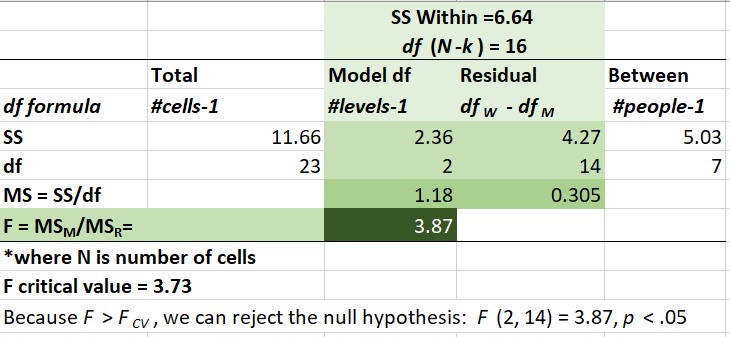
Looking again at our sourcetable, we can move through the steps to calculate our F statistic.
9.4.6 Mean Squares Model & Residual
Now that we have the Sums of Squares, we can calculate the mean squares (we need these for our \(F\) statistic). Here is the formula for the mean square model.
\[MS_M = \frac{SS_{M}}{df^{_{M}}}\]
[1] 1.18HEre is the formula for mean square residual.
And \(MS_R=\) \[MS_R = \frac{SS_{R}}{df^{_{R}}}\] Recall, degrees of freedom for the residual is \(df_w - df_m\). In our case that is 16-2.
[1] 0.3059.4.7 F ratio
The F ratio is calculated with \(MS_M\) and \(MS_R=\).
\[F = \frac{MS_{M}}{MS_{R}}\]
[1] 3.868852To find the \(F_{CV}\) we can use an F distribution table. Or use a look-up function in R, which follows this general form: qf(p, df1, df2. lower.tail=FALSE)
[1] 3.738892Our example has 2 (numerator) and 14 (denominator) degrees of freedom. If we use a table we find the corresponding degrees of freedom combinations for the column where \(\alpha = .05\). We observe that any \(F\) value > 3.73 will be statistically significant. Our \(F\) = 3.87, so we have (just barely) exceeded the threshold. This is our omnibus F. We know there is at least 1 statistically significant difference between our pre, post, and follow-up conditions.
You may notice that the results from the hand calculation are slightly different from the results I will obtain with the R packages. Hand calculations and those used in the R packages likely differ on how the sums of squares is calculated. While the results are “close-ish” they are not always identical.
Should we be concerned? No (and yes). My purpose in teaching hand calculations is for creating a conceptual overview of what is occurring in ANOVA models. If this lesson was a deeper exploration into the inner workings of ANOVA, we would take more time to understand what is occurring. My goal is to provide you with enough of an introduction to ANOVA that you would be able to explore further which sums of squares type would be most appropriate for your unique ANOVA model.
9.5 Working the One-Way Repeated Measures ANOVA with R packages
As usual, we will work through the testing of statistical assumptions, calculating the omnibus, and then (if the omnibus is significant), conducting follow-up tests.
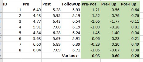
9.5.1 Testing the assumptions
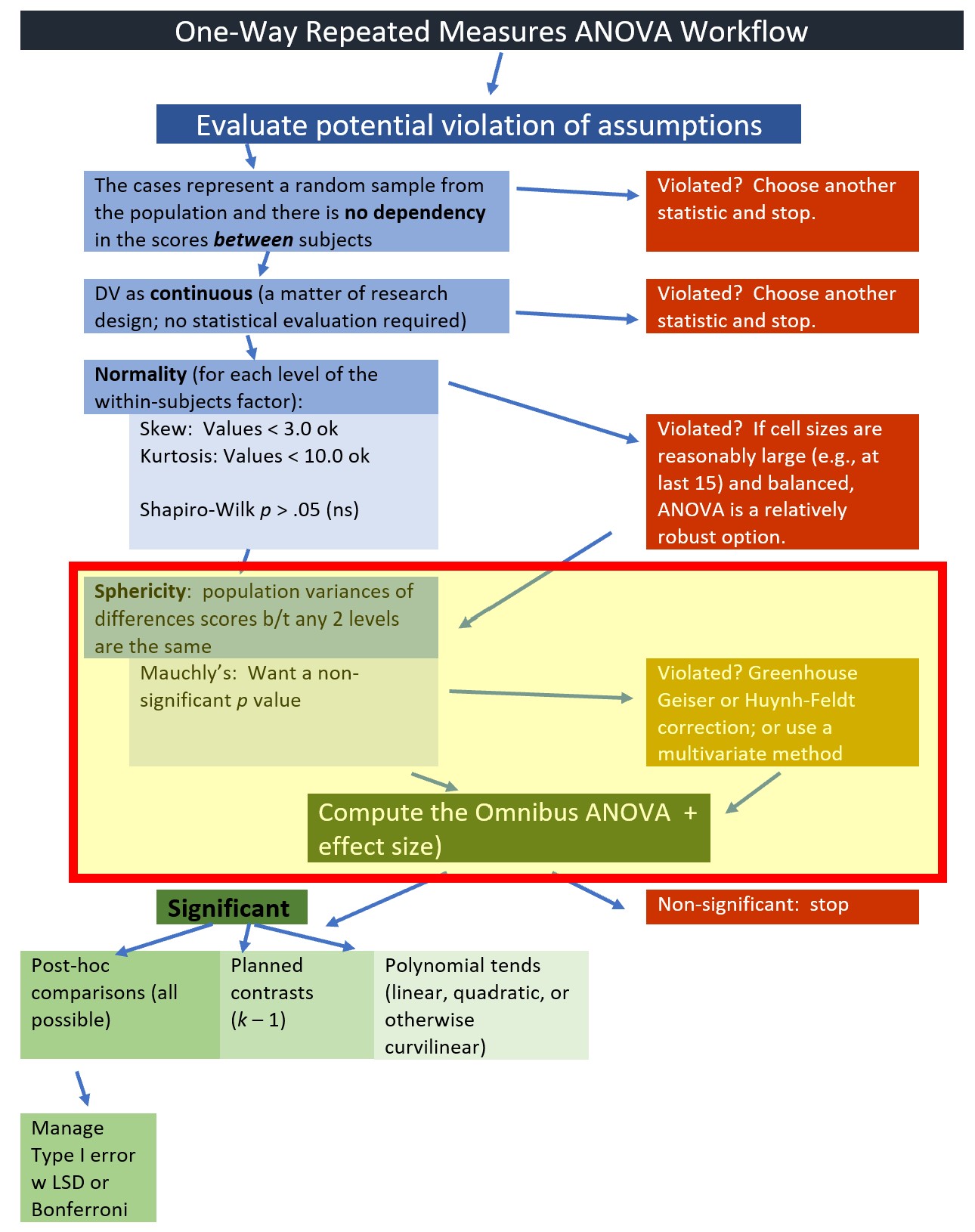
We will start by testing the assumptions. Highlighting in the figure notes our place in the one-way ANOVA workflow:
There are several different ways to conduct a repeated measures ANOVA. Each has different assumptions/requirements. These include:
- univariate statistics
- This is what we will use today.
- multivariate statistics
- Functionally similar to univariate, except the underlying algorithm does not require the sphericity assumption.
- An example of using a multivariate approach to working the problem (using the car package) is in the appendix.
- multi-level modeling/hierarchical linear modeling
- This a different statistic altogether and is addressed in the multilevel modeling OER.
9.5.1.1 Univariate assumptions for repeated measures ANOVA
- The cases represent a random sample from the population.
- There is no dependency in the scores between participants.
- Of course there is intentional dependency in the repeated measures (or within-subjects) factor.
- There are no significant outliers in any cell of the design
- Check by visualizing the data using box plots. The identify_outliers() function in the rstatix package identifies extreme outliers.
- The dependent variable is normally distributed in the population for each level of the within-subjects factor.
- Conduct a Shapiro-Wilk test of normality for each of the levels of the DV.
- Visually examine Q-Q plots.
- The population variance of difference scores computed between any two levels of a within-subjects factor is the same value regardless of which two levels are chosen; termed the sphericity assumption. This assumption is
- akin to compound symmetry (both variances across conditions are equal).
- akin to the homogeneity of variance assumption in between-group designs.
- sometimes called the homogeneity-of-variance-of-differences assumption.
- statistically evaluated with Mauchly’s test. If Mauchly’s p < .05, there are statistically significant differences. The anova_test() function in the rstatix package reports Mauchly’s and two alternatives to the traditional F that correct the values by the degree to which the sphericity assumption is violated.
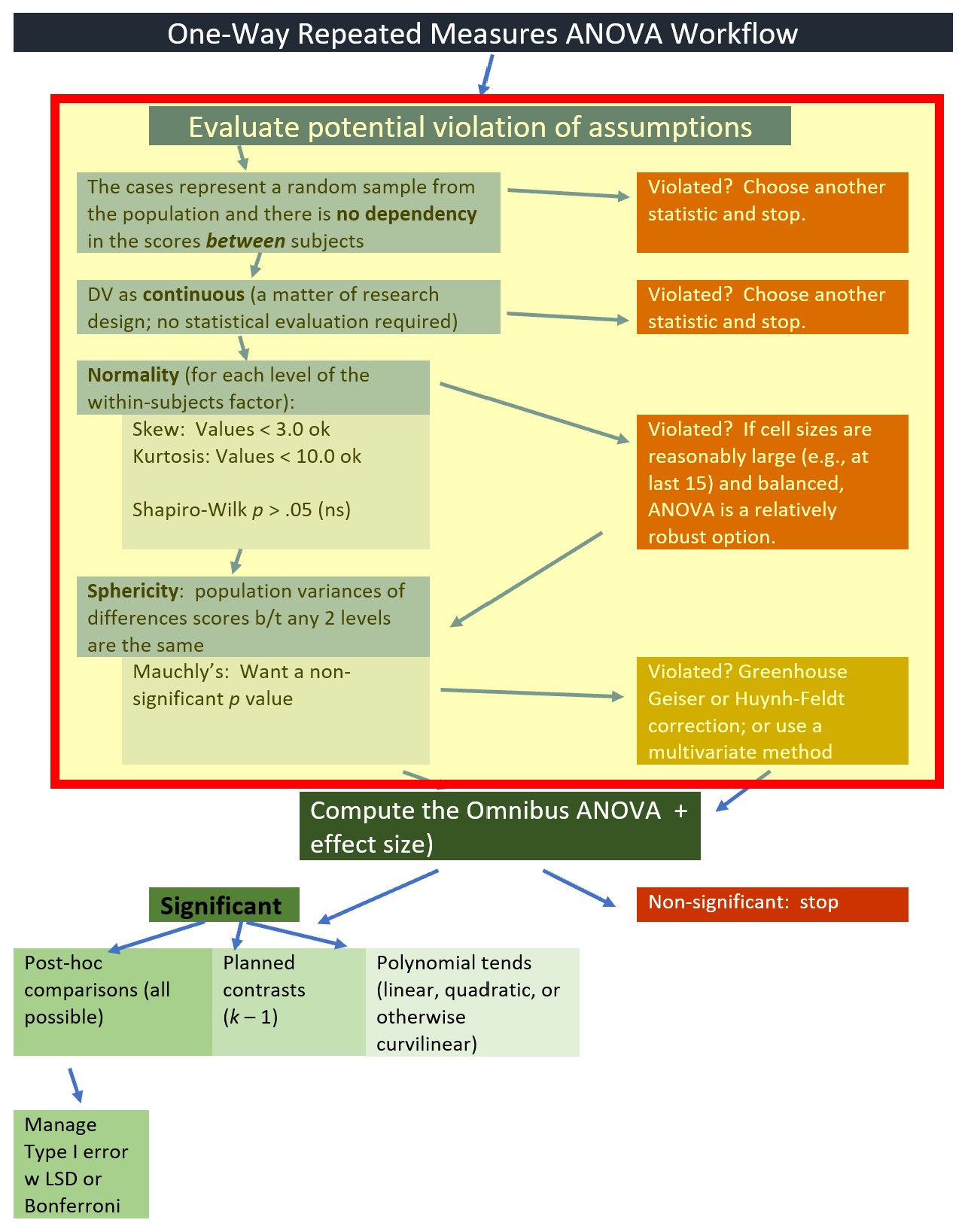
9.5.1.2 Demonstrating sphericity
Using the data from our motivating example, I calculated differences for each of the time variables. These are the three columns (in green shading) on the right. The variance for each is reported at the bottom of the column.
When we get into the analysis, we will use Mauchly’s test in hopes that there are non-significant differences in variances between all three of the comparisons.
We are only concerned with the sphericity assumption if there are three or more groups.
\[variance_{A-B} \approx variance_{A-C}\approx variance_{B-C}\]
9.5.1.3 Is the data normally distributed?
We can obtain skew and kurtosis values for each cell in our model with the psych::describeBy() function.
            item   group1 vars n     mean        sd   median  trimmed       mad
Resilience1    1      Pre    1 8 5.587693 0.8217561 5.770952 5.587693 1.1471137
Resilience2    2     Post    1 8 6.327615 0.6550520 6.356491 6.327615 0.8751431
Resilience3    3 FollowUp    1 8 6.136916 0.4729432 6.215983 6.136916 0.4416578
                 min      max    range       skew  kurtosis        se
Resilience1 4.428839 6.597214 2.168376 -0.1755752 -1.448137 0.2905347
Resilience2 5.283057 7.089591 1.806534 -0.2819094 -1.209000 0.2315959
Resilience3 5.186767 6.708259 1.521491 -0.8802629  0.121247 0.1672107
Our skew and kurtosis values fall below the thresholds of concern (Kline, 2016a):
- < |3| for skew
- < |10| for kurtosis
The Shapiro-Wilk test evaluates the hypothesis that the distribution of the data deviates from a comparable normal distribution. If the test is non-significant (p >.05) the distribution of the sample is not significantly different from a normal distribution. If, however, the test is significant (p < .05), then the sample distribution is significantly different from a normal distribution. The rstatix package can conduct this test for us.
# A tibble: 3 × 4
  Wave     variable   statistic     p
  <fct>    <chr>          <dbl> <dbl>
1 Pre      Resilience     0.919 0.419
2 Post     Resilience     0.941 0.617
3 FollowUp Resilience     0.926 0.480
The p value is > .05 for each of the cells. This provides some assurance that we have not violated the assumption of normality at any level of the design.
The \(p\) values for the distributions of the dependent variable (Resilience) in each wave of the study are all well above .05. This tells us that the Resilience variable does not deviate from a statistically significant distribution at any level (Pre, \(W = 0.929, p = 0.418\); Post, \(p = 0.941, p = 0.617\); FellowUp, \(W = 0.926, p = 0.430\)).
Especially in the more simple “ANOVA’s” I like this form of the Shapiro-Wilk test because it makes it clear that we expect normality within each of the grouping levels. This approach, however, is only appropriate when there are a low number of levels/groupings and there are many data points per group. As models become more complex, researchers should use the model-based option for assessing normality. To do this, we first create an object that tests our research model.
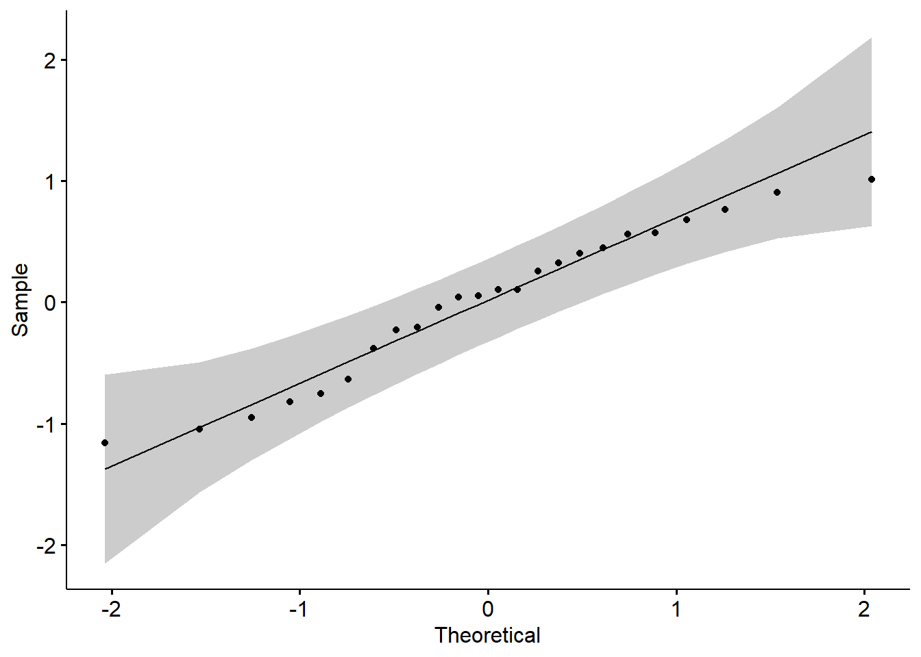
Although that model (a regression model) has information about the results of our primary analysis, at this point we are only using it to investigate the assumption of normality. One product of the analysis is residuals. Residuals are the unexplained variance in the outcome (or dependent) variable after accounting for the predictor (or independent) variable. When we plot these “leftovers” against the values of x, we can visualize the fit of the model in a QQ plot. The dots represent the residuals. When they are relatively close to the line they not only suggest good fit of the model, but we know they are small and evenly distributed around zero (i.e., normally distributed).
We can also use the model in a Shapiro-Wilk test. As before, we want a non-significant result.
# A tibble: 1 × 3
  variable               statistic p.value
  <chr>                      <dbl>   <dbl>
1 residuals(RMres_model)     0.957   0.385
These results are consistent with what we have already learned. That is, the non-significant p value associated with the model-based Shapiro-Wilk test of normality indicates that our distribution of residuals does not differ from a normal distribution (\(W = 0.957, p = 0.385\)). Given the space restrictions in journal articles and the higher priority of describing the results of the primary analyses, I am more likely to report model-level results than the results from the cell-based Shapiro-Wilk tests.
There are limitations to the Shapiro-Wilk test. As the dataset being evaluated gets larger, the Shapiro-Wilk test becomes more sensitive to small deviations; this leads to a greater probability of rejecting the null hypothesis (null hypothesis being the values come from a normal distribution). Green and Salkind (2017c) advised that ANOVA is relatively robust to violations of normality if there are at least 15 cases per cell and the design is reasonably balanced (i.e., equal cell sizes).
9.5.1.4 Are there any outliers (and should we consider their removal)?
The boxplot is one common way for identifying outliers. The boxplot uses the median and the lower (25th percentile) and upper (75th percentile) quartiles. The difference bewteen Q3 and Q1 is the interquartile range (IQR). Outliers are generally identified when values fall outside these lower and upper boundaries:
- Q1 - 1.5xIQR
- Q3 + 1.5xIQR
Extreme values occur when values fall outside these boundaries:
- Q1 - 3xIQR
- Q3 + 3xIQR
Let’s take another look at the boxplot. Swapping “jitter” for “point” may help with the visual inspection.
ggpubr::ggboxplot(Amodeo_long, x = "Wave", y = "Resilience", add = "point", color = "Wave", title = "Figure 9.2 Identifying Outliers with Boxplots")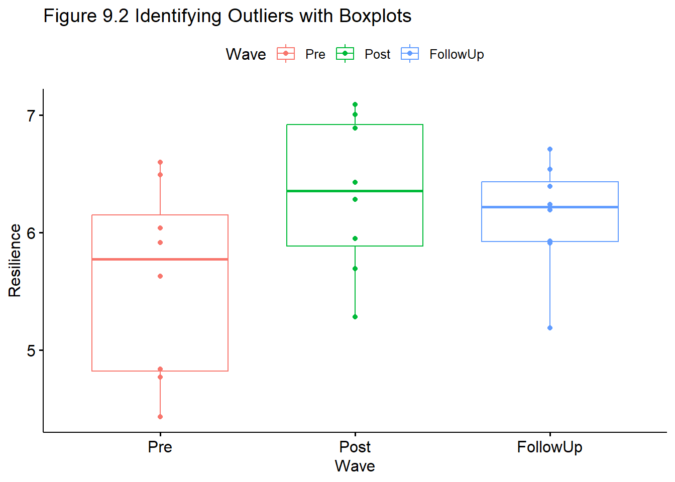
The package rstatix has features that allow us to identify outliers.
[1] Wave       ID         Resilience m_dev      m_devSQ    is.outlier is.extreme
<0 rows> (or 0-length row.names)The output, “0 rows” indicates there are no outliers.
This is consistent with the visual inspection of boxplots (above), where all observed scores fell within the 1.5x the interquartile range. If there were outliers and you chose to delete them, instructions for doing so are found in the parallel sections of the one-way ANOVA and factorial ANOVA lessons.
9.5.1.5 Summarizing results from the analysis of assumptions
Here’s how I would write up the assumptions we have tested thus far:
Similarly, no extreme outliers were identified and results of a model-based Shapiro-Wilk test of normality, indicated that the model residuals did not did differ from a normal distribution \((W = 0.979, p = 0.15)\).
Repeated measures ANOVA has several assumptions regarding normality, outliers, and sphericity. Regarding normality, no values of skew and kurtosis (at each wave of assessment) fell within cautionary ranges for skew and kurtosis (Kline, 2016a). Additionally, results of a model-based Shapiro-Wilk test of normality indicated that the model residuals did not differ from a normal distribution (\(W = 0.957, p = 0.385\)). Visual inspection of boxplots for each wave of the design, assisted by the identify_outliers() function in the rstatix package (which reports values above Q3 + 1.5xIQR or below Q1 - 1.5xIQR, where IQR is the interquartile range) indicated no outliers.
9.5.1.6 Assumption of Sphericity
The sphericity assumption is automatically checked with Mauchley’s test during the computation of the ANOVA when the rstatix::anova_test() function is used. When the rstatix::get_anova_table() function is used, the Greenhouse-Geisser sphericity correction is automatically applied to factors violating the sphericity assumption.
The effect size, \(\eta^2\) is reported in the column labeled “ges.” Conventionally, values of .01, .06, and .14 are considered to be small, medium, and large effect sizes, respectively.
You may see different values (.02, .13, .26) offered as small, medium, and large – these values are used when multiple regression is used. A useful summary of effect sizes, guide to interpreting their magnitudes, and common usage can be found here (Watson, 2020).
Earlier in the lesson I noted that the evaluation of the sphericity assumption occurs at the same time that we evaluate the omnibus ANOVA. We are at that point in the analyses. The workflow points to our stage in the process.
9.5.2 Computing the Test Statistic
As we prepare to run the omnibus ANOVA it may be helpful to think again about our variables. Our DV, Resilience, should be a continuous variable. In R, its structure should be “num.” Our predictor, Wave, should be categorical. In R case, Wave should be an ordered factor that is consistent with its timing: pre, post, follow-up.
The repeated measures ANOVA must be run with a long form of the data. This means that there needs to be a within-subjects identifier. In our case, it is the “ID” variable which is also formatted as a factor.
We can verify the format of our variables by examining the structure of our dataframe. Recall that we created the “m_dev” and “m_devSQ” variables earlier in the demonstration. We will not use them in this analysis; it does not harm anything for them to “ride along” in the dataframe.
'data.frame':   24 obs. of  5 variables:
 $ ID        : Factor w/ 8 levels "1","2","3","4",..: 1 1 1 2 2 2 3 3 3 4 ...
 $ Wave      : Factor w/ 3 levels "Pre","Post","FollowUp": 1 2 3 1 2 3 1 2 3 1 ...
 $ Resilience: num  6.49 5.28 5.93 4.43 5.95 ...
 $ m_dev     : num  0.4747 -0.7344 -0.0895 -1.5886 -0.0689 ...
 $ m_devSQ   : num  0.22536 0.53927 0.00801 2.52355 0.00475 ...
We can use the rstatix::anova_test() function to calculate the omnibus ANOVA. Notice where our variables are included in the script:
- Resilience is the dv
- ID is the wid
- Wave is assigned to within
ANOVA Table (type III tests)

$ANOVA
  Effect DFn DFd    F     p p<.05   ges
1   Wave   2  14 3.91 0.045     * 0.203

$`Mauchly's Test for Sphericity`
  Effect     W     p p<.05
1   Wave 0.566 0.182

$`Sphericity Corrections`
  Effect   GGe    DF[GG] p[GG] p[GG]<.05   HFe      DF[HF] p[HF] p[HF]<.05
1   Wave 0.698 1.4, 9.77 0.068           0.817 1.63, 11.44 0.057
We can assemble our F string from the ANOVA object: \(F(2,14) = 3.91, p = 0.045, \eta^2 = 0.203\)
From the Mauchly’s Test for Sphericity object we learn that we did not violate the sphericity assumption: \(W = 0.566, p = .182\)
From the Sphericity Corrections object are output for two alternative corrections to the F statistic, the Greenhouse-Geiser epsilon (GGe), and Huynh-Feldt epsilon (HFe). Because we did not violate the sphericity assumption we do not need to use them. Notice that these two tests adjust our df (both numerator and denominator) to have a more conservative p value.
If we needed to write an F string that is corrected for violation of the sphericity assumption, it might look like this:
The Greenhouse Geiser estimate was 0.698 the correct omnibus was F(1.4, 9.77) = 3.91, p = .068. The Huyhn Feldt estimate was 0.817 and the corrected omnibus was F (1.63, 11.44) = 3.91 p = .057.
You might be surprised that we are at follow-up already.
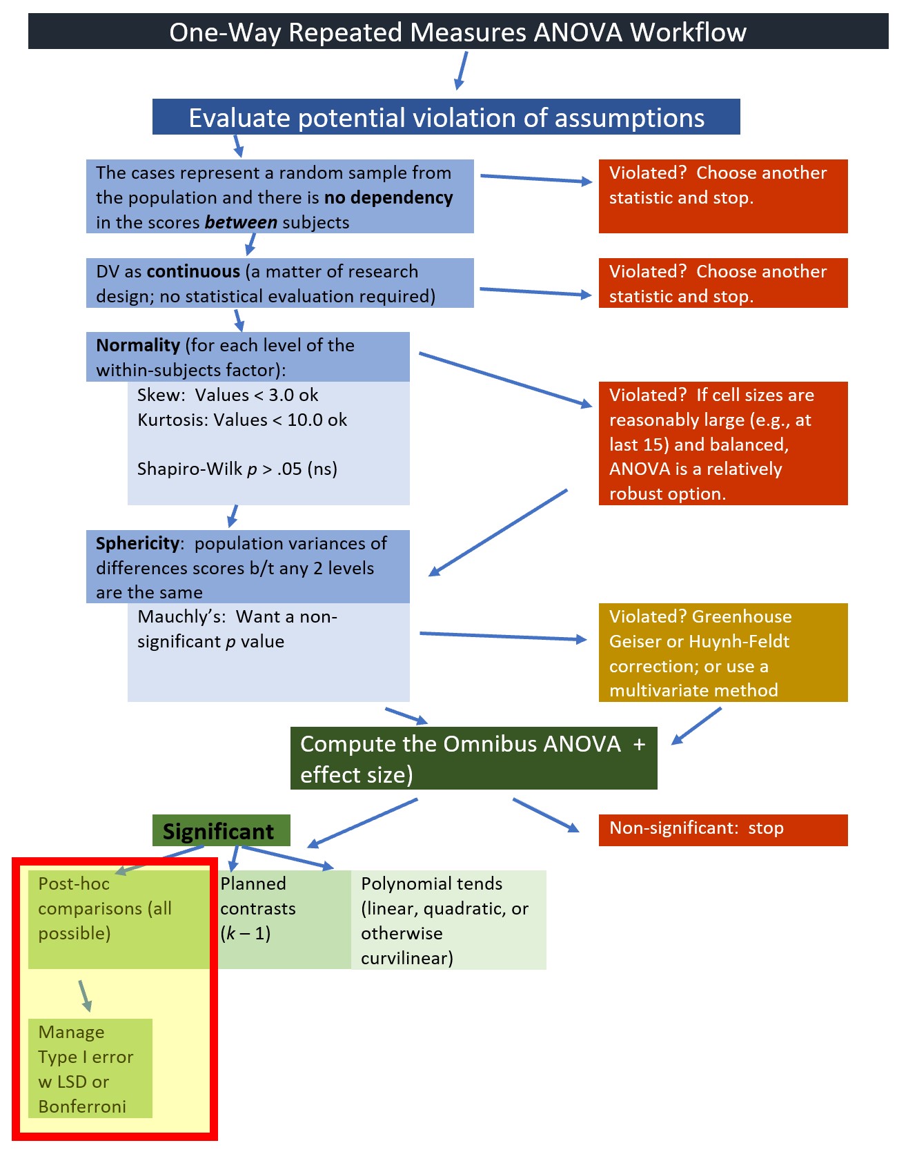 ### Planning for the management of Type I Error
In a one-way repeated measures ANOVA, managing Type I error can be relatively straightforward.
The LSD (least significant differences) method is especially appropriate in the one-way ANOVA scenario when there are only three levels in the factor. In this case, Green and Salkind (2017c) have suggested that alpha can be retained at the alpha level for the “family” (\(\alpha_{family}\)), which is conventionally \(p = .05\) and used both to evaluate the omnibus and, so long as they don’t exceed three in number, the planned or pairwise comparisons that follow. Because there are only three levels (i.e., pre, post, follow-up) in this one-way repeated measures design this is what I will do.
More information about options for managing Type I error is included in the appendix.
9.5.3 Follow-up to Omnibus F
Given the simplicity of our design, it makes sense to me to follow-up with post hoc, pairwise, comparisons. Note that when I am calculating these pairwise t tests, I am creating an object (named “pwc”). The object will be a helpful tool in creating a Figure and an APA Style table.
Note that the script used to produced the figure will pull the symbols from the column labeled, “p.adj.signif.” The rstatix::pairwise_t_test default is the traditional Bonferroni. Therefore, if we want to use the LSD approach, we must “p.adjust.method” as “none.”
pwc <- Amodeo_long %>%
  rstatix::pairwise_t_test(Resilience~Wave, paired = TRUE, p.adjust.method = "none")
pwc
# A tibble: 3 × 10
.y. group1 group2 n1 n2 statistic df p p.adj p.adj.signif
* <chr> <chr> <chr> <int> <int> <dbl> <dbl> <dbl> <dbl> <chr>
1 Resilience Pre Post 8 8 -2.15 7 0.069 0.069 ns
2 Resilience Pre Follow… 8 8 -2.00 7 0.086 0.086 ns
3 Resilience Post Follow… 8 8 1.06 7 0.325 0.325 ns Although omnibus test had a statistically significant result, we did not obtain statistically significant results in an of the posthoc pairwise comparisons. Why not?
- Our omnibus F was right at the margins
- a larger sample size (assuming that the effects would hold) would have been more powerful.
- there could be significance if we compared pre to the combined effects of post and follow-up.
How would we manage Type I error? With only three possible post-omnibus comparisons, I would cite the Tukey LSD approach and not adjust the alpha to a more conservative level (Green & Salkind, 2017c).
We can combine information from the object we created (“bxp”) from an earlier boxplot with the object we saved from the posthoc pairwise comparisons (“pwc) to enhance our boxplot with the F string and indications of pairwise significant (or, in our case, non-significance).
RMbox <- ggpubr::ggboxplot(Amodeo_long, x = "Wave", y = "Resilience", add = "jitter", color = "Wave", title = "Figure 9.3 Resilience as a Function of Wave")
pwc <- pwc %>% rstatix::add_xy_position(x = "Wave")
RMbox <- RMbox+
ggpubr::stat_pvalue_manual(pwc, label = "p.adj.signif", tip.length = 0.01, hide.ns = FALSE, step.increase = 0.05) +
labs(
subtitle = rstatix::get_test_label(RM_AOV, detailed = TRUE),
caption = rstatix:: get_pwc_label(pwc)
)
RMbox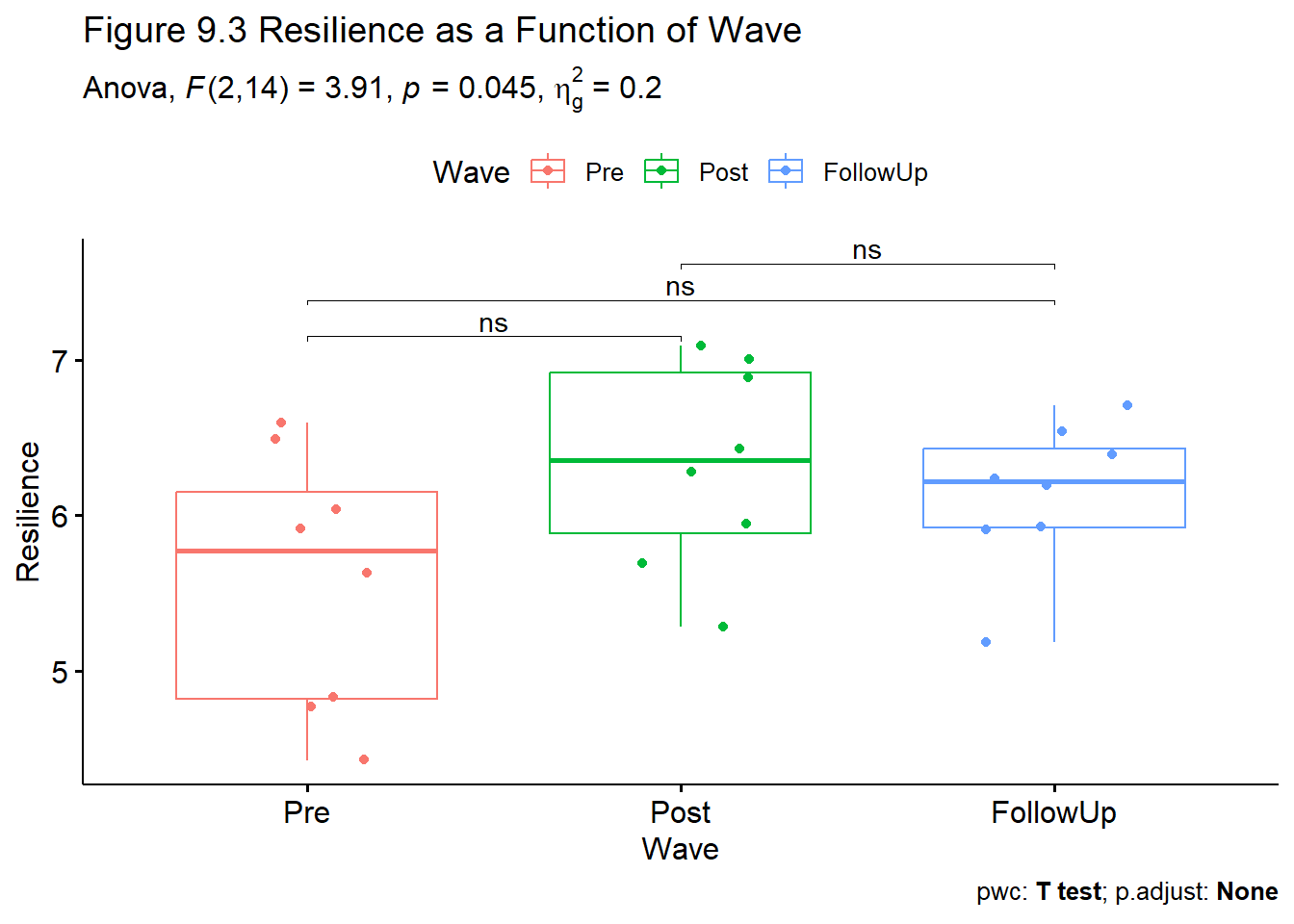 Unfortunately, the apaTables package does not work with the rstatix package, so a table would need to be crafted by hand.
9.6 APA Style Results
Repeated measures ANOVA has several assumptions regarding normality, outliers, and sphericity. Regarding normality, no values of skew and kurtosis (at each wave of assessment) fell within cautionary ranges for skew and kurtosis (Kline, 2016a). Additionally, results of a model-based Shapiro-Wilk test of normality indicated that the model residuals did not differ from a normal distribution (\(W = 0.957, p = 0.385\)). Visual inspection of boxplots for each wave of the design, assisted by the identify_outliers() function in the rstatix package (which reports values above Q3 + 1.5xIQR or below Q1 - 1.5xIQR, where IQR is the interquartile range) indicated no outliers. A non-significant Mauchley’s test (\(W = 0.566, p = .182\)) indicated that the sphericity assumption was not violated.
The omnibus ANOVA was significant: \(F(2,14) = 3.91, p = 0.045, \eta^2 = 0.203\). We followed up with all pairwise comparisons. Curiously, and in spite of a significant omnibus test, there were not statistically significant differences between any of the pairs. Regarding pre versus post, \(t = -2.15, p= .069\). Regarding pre versus follow-up, \(t = -2.00, p = .068\). Regarding post versus follow-up, \(t = 1.059, p = .325\). Because there were only three pairwise comparisons subsequent to the omnibus test, we used the LSD (least significant differences) approach to managing Type I error and alpha was retained at .05 (Green & Salkind, 2017c). While the trajectories from pre-to-post and pre-to-follow-up were in the expected direction, the small sample size likely contributed to a Type II error. Descriptive statistics are reported in Table 1 and the differences are illustrated in Figure 1.
While I have not located a package that will take rstatix output to make an APA style table, we can use the MASS package to write the pwc object to a .csv file, then manually make our own table.
9.6.1 Comparison with Amodeo et al.(2018)
How do our findings and our write-up from the simulated data compare with the original article?
In the published manuscript, the F string is presented in the Table 1 note (\(F[1.612, 11.283]) = 6.390, p = 0.18, \eta _{p}^{2}\)). We can tell from the fractional degrees of freedom that the p value has been had a correction for violation of the sphericity assumption.
Table 1 also reports all of the post hoc, pairwise comparisons. There is no mention of control for Type I error. Had they used a traditional Bonferroni, they would have needed to reduce the alpha to (k*(k-1)/2) and then divide .05 by that number.
[1] 3[1] 0.01666667Although Amodeo et al. report six comparisons; three are repeated because they are merely in reverse. Thus, the revised alpha would be .016 and the one, lone, comparison would not have been statistically significant. That said, the Tukey LSD is appropriate because there are only 3 comparisons and holding alpha at .05 can be defended (Green & Salkind, 2017c).
- Regarding the presentation of the results
- there is no figure
- there is no data presented in the text; all data is presented in Table 1
- Regarding the research design and its limitations
- the authors note that a control condition would have better supported the conclusions
- the authors note the limited sample size and argue that this is a difficult group to recruit for intervention and evaluation
- the article is centered around the qualitative aspect of the design; the quantitative portion is, appropriately, secondary
9.7 Power Analysis
Power analysis allows us to determine the probability of detecting an effect of a given size with a given level of confidence. The package wp.rmanova was designed for power analysis in repeated measures ANOVA.
In the WebPower package, we specify 6 of 7 interrelated elements; the package computes the missing one.
- n = sample size (number of individuals in the whole study).
- ng = number of groups.
- nm = number of measurements/conditions/waves.
- f = Cohen’s f (an effect size; we can use an effect size converter to obtain this value)
- Cohen suggests that f values of 0.1, 0.25, and 0.4 represent small, medium, and large effect sizes, respectively.
- nscor = the Greenhouse Geiser correction from our ouput; 1.0 means no correction was needed and is the package’s default; < 1 means some correction was applied.
- alpha = is the probability of Type I error; we traditionally set this at .05
- power = 1 - P(Type II error) we traditionally set this at .80 (so anything less is less than what we want).
- type = 0 is for between-subjects, 1 is for repeated measures, 2 is for interaction effect.
I used effectsize::eta2_to_f packages convert our \(\eta^2\) to Cohen’s f.
[1] 0.5046832Retrieving the information about our study, we add it to all the arguments except the one we wish to calculate. For power analysis, we write “power = NULL.”
Repeated-measures ANOVA analysis

    n      f ng nm nscor alpha     power
    8 0.5047  1  3 0.689  0.05 0.1619613

NOTE: Power analysis for within-effect test
URL: http://psychstat.org/rmanova
Here we learned that we were only powered at .16. That is, we had a 16% chance of finding a statistically significant effect if, in fact, it existed. This is low!
In reverse, setting power at .80 (the traditional value) and changing n to NULL yields a recommended sample size.
In many cases we won’t know some of the values in advance. We can make best guesses based on our review of the literature.
WebPower::wp.rmanova(n=NULL, ng=1, nm=3, f = .5047, nscor = .689, alpha = .05, power = .80, type = 1)Repeated-measures ANOVA analysis
n f ng nm nscor alpha power
50.87736 0.5047 1 3 0.689 0.05 0.8
NOTE: Power analysis for within-effect test
URL: http://psychstat.org/rmanovaWith these new values, we learn that we would need 50 individuals in order to feel confident in our ability to get a statistically significant result if, in fact, it existed.
9.8 Practice Problems
The suggestions for homework differ in degree of complexity. I encourage you to start with a problem that feels “do-able” and then try at least one more problem that challenges you in some way. All problems attempted should have at least three levels in the independent variable. At least one problem should have a significant omnibus test and require follow-up.
Regardless, your choices should meet you where you are (e.g., in terms of your self-efficacy for statistics, your learning goals, and competing life demands). Whichever you choose, you will focus on these larger steps in one-way repeated measures/within-subjects ANOVA, including:
- test the statistical assumptions
- conduct a one-way, including
- omnibus test and effect size
- conduct follow-up testing
- write a results section to include a figure and tables
9.8.1 Problem #1: Change the Random Seed
If repeated measures ANOVA is new to you, perhaps change the random seed and follow-along with the lesson.
9.8.2 Problem #2: Increase N
Our analysis of the Amodeo et al. (Amodeo et al., 2018) data failed to find significant increases in resilience from pre-to-post through follow-up. Our power analysis suggested that a sample size of 50 would be sufficient to garner statistical significance. The script below re-simulates the data by increasing the sample size to 50 (from 8). All else remains the same.
set.seed(2022)
ID<-factor(c(rep(seq(1,50),each=3)))#gives me 8 numbers, assigning each number 3 consecutive spots, in sequence
Resilience<-rnorm(150,mean=c(5.7,6.21,6.26),sd=c(.88,.79,.37)) #gives me a column of 24 numbers with the specified Ms and SD
Wave<-rep(c("Pre","Post", "FollowUp"),each=1,50) #repeats pre, post, follow-up once each, 8 times
Amodeo50_long<-data.frame(ID, Wave, Resilience)
9.8.3 Problem #3: Try Something Entirely New
Using data for which you have permission and access (e.g., IRB approved data you have collected or from your lab; data you simulate from a published article; data from an open science repository; data from other chapters in this OER), complete a one-way repeated measures ANOVA. Please have at least 3 levels for the predictor variable.
9.8.4 Grading Rubric
Regardless which option(s) you chose, use the elements in the grading rubric to guide you through the practice.
| Assignment Component | Points Possible | Points Earned |
|---|---|---|
| 1. Narrate the research vignette, describing the IV and DV. The data you analyze should have at least 3 levels in the independent variable; at least one of the attempted problems should have a significant omnibus test so that follow-up is required) | 5 | _____ |
| 2. Check and, if needed, format data | 5 | _____ |
| 3. Evaluate statistical assumptions | 5 | _____ |
| 4. Conduct omnibus ANOVA (w effect size) | 5 | _____ |
| 5. Conduct all possible pairwise comparisons (like in the lecture) | 5 | _____ |
| 6. Describe approach for managing Type I error | 5 | _____ |
| 7. APA style results with figure | 5 | _____ |
| 8. Conduct power analyses to determine the power of the current study and a recommended sample size. | 5 | _____ |
| 9. Explanation to grader | 5 | _____ |
| Totals | 40 | _____ |
| Hand Calculations | Points Possible | Points Earned |
|---|---|---|
| 1. Calculate sums of squares total (SST) for the omnibus ANOVA. Steps in this calculation must include calculating a grand mean and creating variables representing the mean deviation and mean deviation squared. | 4 | _____ |
| 2. Calculate the sums of squares within (SSW) for the omnibus ANOVA. A necessary step in this equation is to calculate the variance for each case (student). | 4 | _____ |
| 3. Calculate sums of squares model (SSM) for for the effect of time (or repeated measures). | 4 | _____ |
| 4. Calculate sums of squares residual (SSR). | 4 | _____ |
| 5. Calculate the sums of squares between (SSB). | 4 | _____ |
| 6. Create a source table that includes the sums of squares, degrees of freedom, mean squares, F values, and F critical values | 8 | _____ |
| 6. Are the F-tests statistically significant? Why or why not? | 2 | _____ |
| 7. Assemble the results into a statistical strings | 4 | _____ |
| Totals | 26 | _____ |
9.9 Homeworked Example
For more information about the data used in this homeworked example, please refer to the description and codebook located at the end of the introduction.
9.9.1 Working the Problem with R and R Packages
Narrate the research vignette, describing the IV and DV. The data you analyze should have at least 3 levels in the independent variable; at least one of the attempted problems should have a significant omnibus test so that follow-up is required)
I want to ask the question, do course evaluation ratings for the traditional pedagogy dimension differ for students across the ANOVA, multivariate, and psychometrics courses (in that order, because that’s the order in which the students take the class.)
The dependent variable is the evaluation of traditional pedagogy. The independent variable is course/time (i.e., each student offers course evaluations in each of the three classes).
If you wanted to use this example and dataset as a basis for a homework assignment, the three different classes are the only repeated measures variable. Rather, you could choose a different dependent variable. I chose the traditional pedagogy subscale. Two other subscales include socially responsive pedagogy and valued by the student.
Check and, if needed, format data
The TradPed (traditional pedagogy) variable is an average of the items on that scale. I will first create that variable.
#This code was recently updated and likely differs from the screencasted lecture

#Calculates a mean if at least 75% of the items are non-missing; adjusts the calculating when there is missingness
big$TradPed <- datawizard::row_means(big, select = c('ClearResponsibilities', 'EffectiveAnswers','Feedback', 'ClearOrganization','ClearPresentation'), min_valid = .75)
Let’s trim to just the variables we need.
  deID Course TradPed
1    1  ANOVA     4.4
2    2  ANOVA     3.8
3    3  ANOVA     4.0
4    4  ANOVA     3.0
5    5  ANOVA     4.8
6 6 ANOVA 3.5- Grouping variables: factors
- Dependent variable: numerical or integer
Classes 'data.table' and 'data.frame':  310 obs. of  3 variables:
 $ deID   : int  1 2 3 4 5 6 7 8 9 10 ...
 $ Course : Factor w/ 3 levels "Psychometrics",..: 2 2 2 2 2 2 2 2 2 2 ...
 $ TradPed: num  4.4 3.8 4 3 4.8 3.5 4.6 3.8 3.6 4.6 ...
- attr(*, ".internal.selfref")=<externalptr> rm1wLONG_df$Course <- factor(rm1wLONG_df$Course, levels = c("ANOVA", "Multivariate", "Psychometrics"))
str(rm1wLONG_df)Classes 'data.table' and 'data.frame': 310 obs. of 3 variables:
$ deID : int 1 2 3 4 5 6 7 8 9 10 ...
$ Course : Factor w/ 3 levels "ANOVA","Multivariate",..: 1 1 1 1 1 1 1 1 1 1 ...
$ TradPed: num 4.4 3.8 4 3 4.8 3.5 4.6 3.8 3.6 4.6 ...
- attr(*, ".internal.selfref")=<externalptr> Let’s update the df to have only complete cases.
[1] 307This took us to 307 cases.
These analyses require that students have completed evaluations for all three courses. In the lesson, I restructured the data from long, to wide, back to long again. While this was useful pedagogy in understanding the difference between the two data structures, there is also super quick code that will simply retain data that has at least three observations per student.
This took the data to 210 observations. Since each student contributed 3 observations, we know \(N = 70\).
[1] 70Before we start, let’s get a plot of what’s happening:
bxp <- ggpubr::ggboxplot(rm1wLONG_df, x = "Course", y = "TradPed", add = "point", color = "Course",
    xlab = "Statistics Course", ylab = "Traditional Pedagogy Course Eval Ratings", title = "Course Evaluations across Doctoral Statistics Courses")
bxp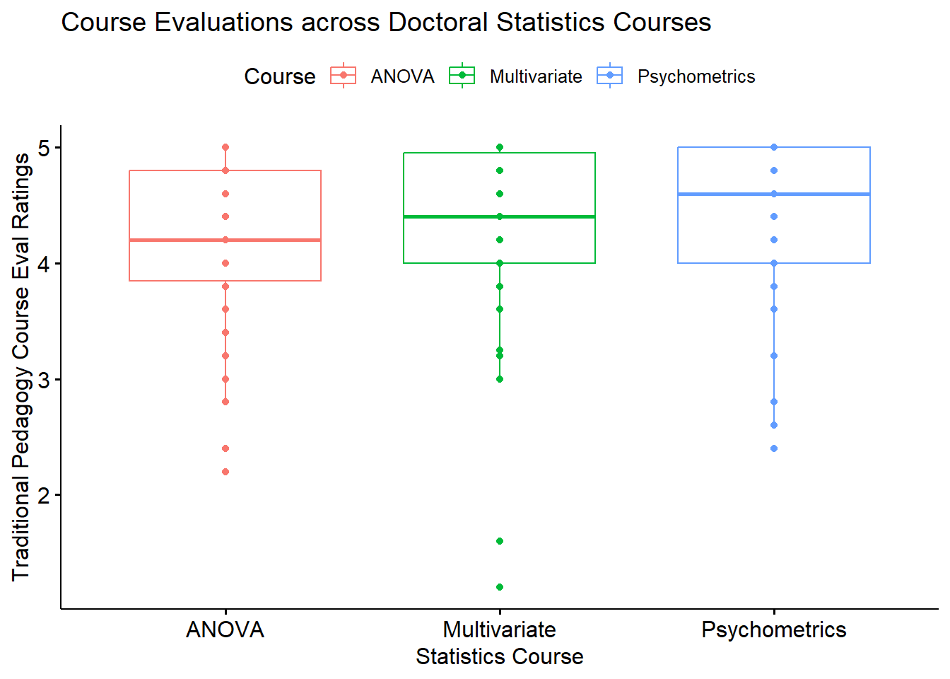
Evaluate statistical assumptions
Is the dependent variable normally distributed?
Given that this is a one-way repeated measures ANOVA model, the dependent variable must be normally distributed within each of the cells of the factor.
We can examine skew and kurtosis in each of the levels of the TradPed variable with psych::describeBy().
#R wasn't recognizing the data, so I quickly applied the as.data.frame function
rm1wLONG_df <- as.data.frame(rm1wLONG_df)
psych::describeBy(TradPed ~ Course, mat = TRUE, type = 1, data = rm1wLONG_df)
item group1 vars n mean sd median trimmed mad
TradPed1 1 ANOVA 1 70 4.211429 0.7108971 4.2 4.296429 0.88956
TradPed2 2 Multivariate 1 70 4.332143 0.7267176 4.4 4.453571 0.59304
TradPed3 3 Psychometrics 1 70 4.414286 0.6718535 4.6 4.532143 0.59304
min max range skew kurtosis se
TradPed1 2.2 5 2.8 -0.7864361 -0.008737723 0.08496846
TradPed2 1.2 5 3.8 -2.0368575 5.752276032 0.08685937
TradPed3 2.4 5 2.6 -1.3145875 1.306390888 0.08030186Although we note some skew and kurtosis, particularly for the multivariate class, none exceed the critical thresholds of |3| for skew and |10| identified by Kline (2016a).
I can formally test for normality with the Shapiro-Wilk test. If I use the residuals from an evaluated model, with one test, I can determine if TradPed is distributed normally within each of the courses.
Call:
lm(formula = TradPed ~ Course, data = rm1wLONG_df)

Residuals:
     Min       1Q   Median       3Q      Max
-3.13214 -0.33214  0.06786  0.58571  0.78857

Coefficients:
                    Estimate Std. Error t value            Pr(>|t|)
(Intercept)          4.21143    0.08409  50.083 <0.0000000000000002 ***
CourseMultivariate   0.12071    0.11892   1.015              0.3112
CoursePsychometrics  0.20286    0.11892   1.706              0.0895 .
---
Signif. codes:  0 '***' 0.001 '**' 0.01 '*' 0.05 '.' 0.1 ' ' 1

Residual standard error: 0.7035 on 207 degrees of freedom
Multiple R-squared:  0.01403,   Adjusted R-squared:  0.004501
F-statistic: 1.472 on 2 and 207 DF,  p-value: 0.2317
We will ignore this for now, but use the residuals in the formal Shapiro-Wilk test.
# A tibble: 1 × 3
  variable                 statistic  p.value
  <chr>                        <dbl>    <dbl>
1 residuals(RMres_TradPed)     0.876 4.11e-12
The distribution of model residuals is statistically significantly different than a normal distribution \((W = 0.876, p < .001)\). Although we have violated the assumption of normality, ANOVA models are relatively robust to such a violation when cell sizes are roughly equal and greater than 15 each (Green & Salkind, 2017b).
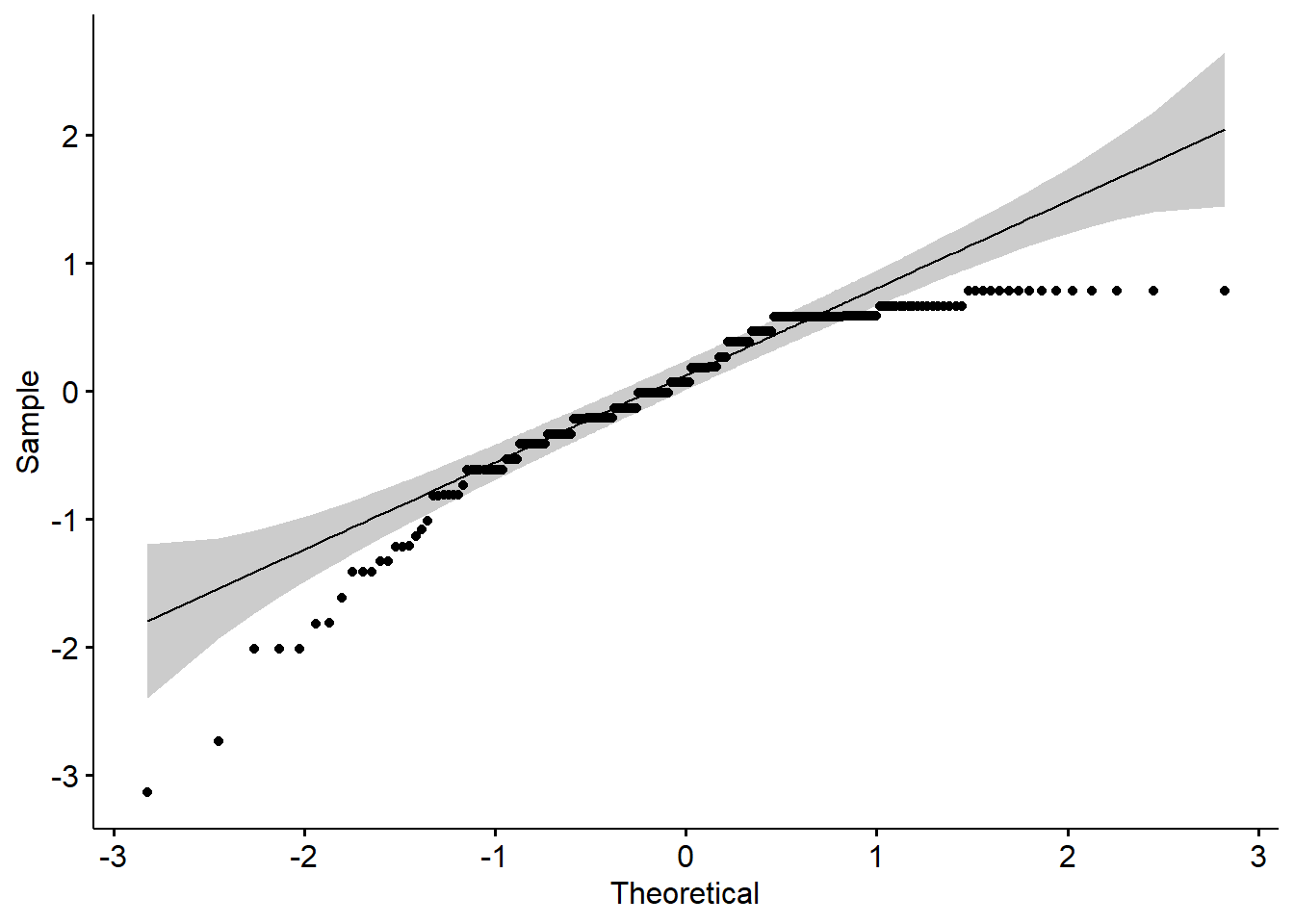
Creating a QQ plot can let us know how badly the distribution departs from a normal one.
We can identify outliers and see if they are reasonable or should be removed.
# A tibble: 6 × 5
  Course         deID TradPed is.outlier is.extreme
  <fct>         <int>   <dbl> <lgl>      <lgl>
1 ANOVA            16     2.2 TRUE       FALSE
2 ANOVA            29     2.4 TRUE       FALSE
3 Multivariate     51     1.2 TRUE       FALSE
4 Multivariate     61     1.6 TRUE       FALSE
5 Psychometrics    11     2.4 TRUE       FALSE
6 Psychometrics    16     2.4 TRUE       FALSE
Outliers for the TradPed variable are among the lowest evaluations (these can be seen on the boxplot). Although there are six outliers identified, none are extreme. Although they contribute to non-normality, I think it’s important that this sentiment be retained in the dataset.
Assumption of sphericity
We will need to evaluate and include information about violations related to sphericity. Because these are calculated at the same time as the ANOVA, itself, I will simply leave this here as a placeholder.
Here’s how I would write up the evaluation of assumptions so far:
We utilized one-way repeated measures ANOVA to determine if there were differences in students’ evaluation of traditional pedagogy across three courses – ANOVA, multivariate, and psychometrics – taught in that order.
Repeated measures ANOVA has several assumptions regarding normality, outliers, and sphericity. Although we note some skew and kurtosis, particularly for the multivariate class, none exceed the critical thresholds of |3| for skew and |10| identified by Kline (2016a). We formally evaluated the normality assumption with the Shapiro-Wilk test. The distribution of model residuals was statistically significantly different than a normal distribution \((W = 0.876, p < .001)\). Although we violated the assumption of normality, ANOVA models are relatively robust to such a violation when cell sizes are roughly equal and greater than 15 each (Green & Salkind, 2017b). Although our data included six outliers, none were classified as extreme. Because they represented lower course evaluations, we believed it important to retain them in the dataset. PLACEHOLDER FOR SPHERICITY.
Conduct omnibus ANOVA (w effect size)
ANOVA Table (type III tests)

$ANOVA
  Effect DFn DFd     F     p p<.05   ges
1 Course   2 138 2.838 0.062       0.014

$`Mauchly's Test for Sphericity`
  Effect     W     p p<.05
1 Course 0.878 0.012     *

$`Sphericity Corrections`
  Effect   GGe       DF[GG] p[GG] p[GG]<.05   HFe       DF[HF] p[HF] p[HF]<.05
1 Course 0.891 1.78, 122.98 0.068           0.913 1.83, 126.02 0.067
Let’s start first with the sphericity test. Mauchly’s test for sphericity was statistically significant, \((W = 0.878, p = 0.012)\). Had we not violated the assumption, our F string would have been created from the data in the ANOVA section of the output : \(F(2, 138) = 2.838, p = 0.062, \eta^2 = 0.14\) However, because we violated the assumption, we need to use the degrees-of-freedom adjusted output under the “Sphericity Corrections” section; \(F(1.78, 122.98) = 2.838, p = 0.068, ges = 0.014\).
While the ANOVA is non-significant, because this is a homework demonstration, I will behave as if the test is significant and continue with the pairwise comparisons.
Conduct all possible pairwise comparisons (like in the lecture)
I will follow up with a test of all possible pairwise comparisons and adjust with the bonferroni.
pwc <- rstatix::pairwise_t_test(TradPed ~ Course, paired = TRUE, p.adjust.method = "bonf", data = rm1wLONG_df)
pwc
# A tibble: 3 × 10
.y. group1 group2 n1 n2 statistic df p p.adj p.adj.signif
* <chr> <chr> <chr> <int> <int> <dbl> <dbl> <dbl> <dbl> <chr>
1 TradPed ANOVA Multi… 70 70 -1.21 69 0.229 0.687 ns
2 TradPed ANOVA Psych… 70 70 -2.07 69 0.043 0.128 ns
3 TradPed Multivari… Psych… 70 70 -0.772 69 0.443 1 ns Consistent with the non-significant omnibus, there were non-significant differences between the pairs. This included, ANOVA and multivariate \((t[69] = -1.215, p = 0.687)\); ANOVA and psychometrics courses \((t[69] = -2.065, p = 0.128)\); and multivariate and psychometrics \((t[69] = -0.772, p = 1.000)\).
Describe approach for managing Type I error
I used a traditional Bonferroni for the three, follow-up, pairwise comparisons.
APA style results with figure
We utilized one-way repeated measures ANOVA to determine if there were differences in students’ evaluation of traditional pedagogy across three courses – ANOVA, multivariate, and psychometrics – taught in that order.
Repeated measures ANOVA has several assumptions regarding normality, outliers, and sphericity. Although we note some skew and kurtosis, particularly for the multivariate class, none exceed the critical thresholds of |3| for skew and |10| identified by Kline (2016a). We formally evaluated the normality assumption with the Shapiro-Wilk test. The distribution of model residuals was statistically significantly different than a normal distribution \((W = 0.876, p < .001)\). Although we violated the assumption of normality, ANOVA models are relatively robust to such a violation when cell sizes are roughly equal and greater than 15 each (Green & Salkind, 2017b). Although our data included six outliers, none were classified as extreme. Because they represented lower course evaluations, we believed it important to retain them in the dataset. Mauchly’s test indicated a violation of the sphericity assumption \((W = 0.878, p = 0.012)\).
Given the violation of the homogeneity of sphericity assumption, we are reporting the Greenhouse-Geyser adjusted values. Results of the omnibus ANOVA were not statistically significant \(F(1.78, 122.98) = 2.838, p = 0.068, ges = 0.014\).
Although we would normally not follow-up a non-significant omnibus ANOVA with more testing, because this is a homework demonstration, we will follow-up the ANOVA with pairwise comparisons and manage Type I error with the traditional Bonferroni approach. Consistent with the non-significant omnibus, there were non-significant differences between the pairs. This included, ANOVA and multivariate \((t[69] = -1.215, p = 0.687)\); ANOVA and psychometrics courses \((t[69] = -2.065, p = 0.128)\); and multivariate and psychometrics \((t[69] = -0.772, p = 1.000)\).
I can update the figure to include star bars.
library(tidyverse)
pwc <- pwc %>%
    rstatix::add_xy_position(x = "Course")
bxp <- bxp + ggpubr::stat_pvalue_manual(pwc, label = "p.adj.signif", tip.length = 0.01, hide.ns = FALSE, y.position = c(5.25, 5.5, 5.75))
bxp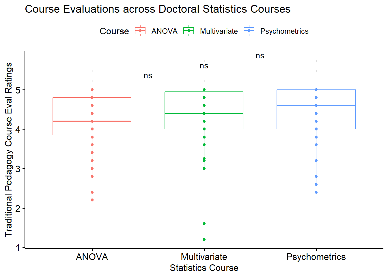
Conduct power analyses to determine the power of the current study and a recommended sample size
In the WebPower package, we specify 6 of 7 interrelated elements; the package computes the missing one.
- n = sample size (number of individuals in the whole study).
- ng = number of groups.
- nm = number of measurements/conditions/waves.
- f = Cohen’s f (an effect size; we can use an effect size converter to obtain this value)
- Cohen suggests that f values of 0.1, 0.25, and 0.4 represent small, medium, and large effect sizes, respectively.
- nscor = the Greenhouse Geiser correction from our ouput; 1.0 means no correction was needed and is the package’s default; < 1 means some correction was applied.
- alpha = is the probability of Type I error; we traditionally set this at .05
- power = 1 - P(Type II error) we traditionally set this at .80 (so anything less is less than what we want).
- type = 0 is for between-subjects, 1 is for repeated measures, 2 is for interaction effect.
I used effectsize::eta2_to_f packages convert our \(\eta^2\) to Cohen’s f.
[1] 0.1191586Retrieving the information about our study, we add it to all the arguments except the one we wish to calculate. For power analysis, we write “power = NULL.”
WebPower::wp.rmanova(n=70, ng=1, nm=3, f = .1192, nscor = .891, alpha = .05, power = NULL, type = 1)Repeated-measures ANOVA analysis
n f ng nm nscor alpha power
70 0.1192 1 3 0.891 0.05 0.1256669
NOTE: Power analysis for within-effect test
URL: http://psychstat.org/rmanovaThe study had a power of 13%. That is, we had a 13% probability of finding a statistically significant result if one existed.
In reverse, setting power at .80 (the traditional value) and changing n to NULL yields a recommended sample size.
WebPower::wp.rmanova(n=NULL, ng=1, nm=3, f = .1192, nscor = .891, alpha = .05, power = .80, type = 1)Repeated-measures ANOVA analysis
n f ng nm nscor alpha power
736.7714 0.1192 1 3 0.891 0.05 0.8
NOTE: Power analysis for within-effect test
URL: http://psychstat.org/rmanovaWith these new values, we learn that we would need 737 individuals in order to obtain a statistically significant result 80% of the time.
9.9.2 Hand Calculations
For hand calculations, I will use the same dataframe (rm1wLONG_df) as I did for the calculations with R and R packages.Before we continue:
You may notice that the results from the hand calculation are slightly different from the results I will obtain with the R packages. This was true in the lesson as well. Hand calculations and those used in the R packages likely differ on how the sums of squares is calculated. While the results are “close-ish” they are not always identical.
Should we be concerned? No (and yes). My purpose in teaching hand calculations is for creating a conceptual overview of what is occurring in ANOVA models. If this lesson was a deeper exploration into the inner workings of ANOVA, we would take more time to understand what is occurring. My goal is to provide you with enough of an introduction to ANOVA that you would be able to explore further which sums of squares type would be most appropriate for your unique ANOVA model.
Calculate sums of squares total (SST) for the omnibus ANOVA. Steps in this calculation must include calculating a grand mean and creating variables representing the mean deviation and mean deviation squared
The formula for sums of squares total: \[SS_{T}= \sum (x_{i}-\bar{x}_{grand})^{2}\].
We can use the mean function from base R to calculate the grand mean:
[1] 4.319286I will create a mean deviation variable by subtracting the mean from each score:
rm1wLONG_df$mDev <- rm1wLONG_df$TradPed - 4.319286
head(rm1wLONG_df)#shows first six rows of dataset
deID Course TradPed mDev
1 11 Psychometrics 2.4 -1.919286
2 12 Psychometrics 4.8 0.480714
3 13 Psychometrics 4.8 0.480714
4 14 Psychometrics 3.2 -1.119286
5 15 Psychometrics 3.6 -0.719286
6 16 Psychometrics 2.4 -1.919286Now I will square the mean deviation:
rm1wLONG_df$mDev2 <- rm1wLONG_df$mDev * rm1wLONG_df$mDev
head(rm1wLONG_df)#shows first six rows of dataset
deID Course TradPed mDev mDev2
1 11 Psychometrics 2.4 -1.919286 3.6836587
2 12 Psychometrics 4.8 0.480714 0.2310859
3 13 Psychometrics 4.8 0.480714 0.2310859
4 14 Psychometrics 3.2 -1.119286 1.2528011
5 15 Psychometrics 3.6 -0.719286 0.5173723
6 16 Psychometrics 2.4 -1.919286 3.6836587Sums of squares total is the sum of the mean deviation squared scores.
[1] 103.9144The sums of squares total is 103.9144.
Calculate the sums of squares within (SSW) for the omnibus ANOVA. A necessary step in this equation is to calculate the variance for each student
Here is the formula for sums of squares within:
\[SS_W = s_{person1}^{2}(n_{1}-1)+s_{person2}^{2}(n_{2}-1)+s_{person3}^{2}(n_{3}-1)+...+s_{personk}^{2}(n_{k}-1)\]
I can get the use the psych::describeBy() to obtain the standard deviations for each student’s three ratings. I can square each of those for the variance to enter into the formula.
          item group1 vars n     mean        sd median  trimmed     mad  min
TradPed1     1     11    1 3 3.400000 0.8717798    3.8 3.400000 0.29652 2.40
TradPed2     2     12    1 3 4.666667 0.4163332    4.8 4.666667 0.29652 4.20
TradPed3     3     13    1 3 4.400000 0.6928203    4.8 4.400000 0.00000 3.60
TradPed4     4     14    1 3 3.600000 0.4000000    3.6 3.600000 0.59304 3.20
TradPed5     5     15    1 3 3.733333 0.4163332    3.6 3.733333 0.29652 3.40
TradPed6     6     16    1 3 2.533333 0.4163332    2.4 2.533333 0.29652 2.20
TradPed7     7     17    1 3 4.600000 0.5291503    4.8 4.600000 0.29652 4.00
TradPed8     8     18    1 3 4.400000 0.5291503    4.6 4.400000 0.29652 3.80
TradPed9     9     19    1 3 4.133333 0.7023769    4.2 4.133333 0.88956 3.40
TradPed10   10     23    1 3 4.733333 0.4618802    5.0 4.733333 0.00000 4.20
TradPed11   11     24    1 3 3.866667 0.4163332    4.0 3.866667 0.29652 3.40
TradPed12   12     25    1 3 4.933333 0.1154701    5.0 4.933333 0.00000 4.80
TradPed13   13     26    1 3 4.733333 0.3055050    4.8 4.733333 0.29652 4.40
TradPed14   14     28    1 3 4.933333 0.1154701    5.0 4.933333 0.00000 4.80
TradPed15   15     29    1 3 3.733333 1.2220202    4.0 3.733333 1.18608 2.40
TradPed16   16     30    1 3 4.666667 0.4163332    4.8 4.666667 0.29652 4.20
TradPed17   17     31    1 3 3.666667 0.9018500    3.6 3.666667 1.18608 2.80
TradPed18   18     32    1 3 4.533333 0.5033223    4.6 4.533333 0.59304 4.00
TradPed19   19     33    1 3 4.000000 0.0000000    4.0 4.000000 0.00000 4.00
TradPed20   20     34    1 3 4.066667 0.9451631    4.4 4.066667 0.59304 3.00
TradPed21   21     39    1 3 3.733333 1.0066446    3.6 3.733333 1.18608 2.80
TradPed22   22     40    1 3 4.933333 0.1154701    5.0 4.933333 0.00000 4.80
TradPed23   23     41    1 3 4.666667 0.3055050    4.6 4.666667 0.29652 4.40
TradPed24   24     43    1 3 4.200000 0.3464102    4.4 4.200000 0.00000 3.80
TradPed25   25     46    1 3 3.883333 0.5484828    4.2 3.883333 0.00000 3.25
TradPed26   26     47    1 3 4.133333 0.1154701    4.2 4.133333 0.00000 4.00
TradPed27   27     48    1 3 4.933333 0.1154701    5.0 4.933333 0.00000 4.80
TradPed28   28     51    1 3 2.933333 1.6165808    3.2 2.933333 1.77912 1.20
TradPed29   29     52    1 3 3.733333 0.1154701    3.8 3.733333 0.00000 3.60
TradPed30   30     53    1 3 4.266667 0.3055050    4.2 4.266667 0.29652 4.00
TradPed31   31     54    1 3 4.800000 0.3464102    5.0 4.800000 0.00000 4.40
TradPed32   32     55    1 3 4.200000 0.9165151    4.4 4.200000 0.88956 3.20
TradPed33   33     56    1 3 3.466667 0.4163332    3.6 3.466667 0.29652 3.00
TradPed34   34     58    1 3 4.533333 0.4163332    4.4 4.533333 0.29652 4.20
TradPed35   35     60    1 3 4.800000 0.3464102    5.0 4.800000 0.00000 4.40
TradPed36   36     61    1 3 2.333333 0.6429101    2.6 2.333333 0.29652 1.60
TradPed37   37     62    1 3 4.600000 0.3464102    4.4 4.600000 0.00000 4.40
TradPed38   38     63    1 3 4.600000 0.5291503    4.8 4.600000 0.29652 4.00
TradPed39   39     64    1 3 3.666667 0.1154701    3.6 3.666667 0.00000 3.60
TradPed40   40     65    1 3 4.866667 0.2309401    5.0 4.866667 0.00000 4.60
TradPed41   41     66    1 3 4.933333 0.1154701    5.0 4.933333 0.00000 4.80
TradPed42   42     67    1 3 4.200000 0.9165151    4.4 4.200000 0.88956 3.20
TradPed43   43     68    1 3 4.933333 0.1154701    5.0 4.933333 0.00000 4.80
TradPed44   44     69    1 3 4.000000 0.5291503    4.2 4.000000 0.29652 3.40
TradPed45   45     70    1 3 4.400000 0.5291503    4.2 4.400000 0.29652 4.00
TradPed46   46     71    1 3 4.400000 0.5291503    4.2 4.400000 0.29652 4.00
TradPed47   47     72    1 3 4.800000 0.3464102    5.0 4.800000 0.00000 4.40
TradPed48   48     73    1 3 4.933333 0.1154701    5.0 4.933333 0.00000 4.80
TradPed49   49     74    1 3 4.866667 0.2309401    5.0 4.866667 0.00000 4.60
TradPed50   50     75    1 3 4.866667 0.2309401    5.0 4.866667 0.00000 4.60
TradPed51   51     76    1 3 5.000000 0.0000000    5.0 5.000000 0.00000 5.00
TradPed52   52     77    1 3 4.000000 0.2000000    4.0 4.000000 0.29652 3.80
TradPed53   53     78    1 3 4.066667 0.1154701    4.0 4.066667 0.00000 4.00
TradPed54   54     79    1 3 4.466667 0.5033223    4.4 4.466667 0.59304 4.00
TradPed55   55     80    1 3 4.333333 0.3055050    4.4 4.333333 0.29652 4.00
TradPed56   56     81    1 3 5.000000 0.0000000    5.0 5.000000 0.00000 5.00
TradPed57   57     82    1 3 4.866667 0.2309401    5.0 4.866667 0.00000 4.60
TradPed58   58     83    1 3 4.733333 0.4618802    5.0 4.733333 0.00000 4.20
TradPed59   59     84    1 3 4.133333 0.4163332    4.0 4.133333 0.29652 3.80
TradPed60   60     86    1 3 4.733333 0.3055050    4.8 4.733333 0.29652 4.40
TradPed61   61     87    1 3 4.600000 0.4000000    4.6 4.600000 0.59304 4.20
TradPed62   62    115    1 3 4.600000 0.3464102    4.8 4.600000 0.00000 4.20
TradPed63   63    116    1 3 3.733333 0.8326664    4.0 3.733333 0.59304 2.80
TradPed64   64    117    1 3 4.333333 0.5773503    4.0 4.333333 0.00000 4.00
TradPed65   65    118    1 3 4.000000 0.0000000    4.0 4.000000 0.00000 4.00
TradPed66   66    124    1 3 4.800000 0.2000000    4.8 4.800000 0.29652 4.60
TradPed67   67    136    1 3 4.533333 0.3055050    4.6 4.533333 0.29652 4.20
TradPed68   68    137    1 3 4.200000 0.3464102    4.0 4.200000 0.00000 4.00
TradPed69   69    138    1 3 4.733333 0.4618802    5.0 4.733333 0.00000 4.20
TradPed70   70    139    1 3 4.533333 0.3055050    4.6 4.533333 0.29652 4.20
          max range               skew kurtosis         se
TradPed1  4.0  1.60 -0.665468866123835     -1.5 0.50332230
TradPed2  5.0  0.80 -0.528004979218190     -1.5 0.24037009
TradPed3  4.8  1.20 -0.707106781186550     -1.5 0.40000000
TradPed4  4.0  0.80  0.000000000000000     -1.5 0.23094011
TradPed5  4.2  0.80  0.528004979218188     -1.5 0.24037009
TradPed6  3.0  0.80  0.528004979218190     -1.5 0.24037009
TradPed7  5.0  1.00 -0.595170064139495     -1.5 0.30550505
TradPed8  4.8  1.00 -0.595170064139495     -1.5 0.30550505
TradPed9  4.8  1.40 -0.172800544078648     -1.5 0.40551750
TradPed10 5.0  0.80 -0.707106781186547     -1.5 0.26666667
TradPed11 4.2  0.80 -0.528004979218188     -1.5 0.24037009
TradPed12 5.0  0.20 -0.707106781186557     -1.5 0.06666667
TradPed13 5.0  0.60 -0.381801774160605     -1.5 0.17638342
TradPed14 5.0  0.20 -0.707106781186557     -1.5 0.06666667
TradPed15 4.8  2.40 -0.381801774160607     -1.5 0.70553368
TradPed16 5.0  0.80 -0.528004979218190     -1.5 0.24037009
TradPed17 4.6  1.80  0.135061522784740     -1.5 0.52068331
TradPed18 5.0  1.00 -0.239063146929544     -1.5 0.29059326
TradPed19 4.0  0.00                NaN      NaN 0.00000000
TradPed20 4.8  1.80 -0.567316577993728     -1.5 0.54569018
TradPed21 4.8  2.00  0.239063146929544     -1.5 0.58118653
TradPed22 5.0  0.20 -0.707106781186557     -1.5 0.06666667
TradPed23 5.0  0.60  0.381801774160605     -1.5 0.17638342
TradPed24 4.4  0.60 -0.707106781186547     -1.5 0.20000000
TradPed25 4.2  0.95 -0.707106781186547     -1.5 0.31666667
TradPed26 4.2  0.20 -0.707106781186557     -1.5 0.06666667
TradPed27 5.0  0.20 -0.707106781186557     -1.5 0.06666667
TradPed28 4.4  3.20 -0.294799620144829     -1.5 0.93333333
TradPed29 3.8  0.20 -0.707106781186552     -1.5 0.06666667
TradPed30 4.6  0.60  0.381801774160605     -1.5 0.17638342
TradPed31 5.0  0.60 -0.707106781186544     -1.5 0.20000000
TradPed32 5.0  1.80 -0.381801774160607     -1.5 0.52915026
TradPed33 3.8  0.80 -0.528004979218190     -1.5 0.24037009
TradPed34 5.0  0.80  0.528004979218190     -1.5 0.24037009
TradPed35 5.0  0.60 -0.707106781186544     -1.5 0.20000000
TradPed36 2.8  1.20 -0.630903856710625     -1.5 0.37118429
TradPed37 5.0  0.60  0.707106781186544     -1.5 0.20000000
TradPed38 5.0  1.00 -0.595170064139495     -1.5 0.30550505
TradPed39 3.8  0.20  0.707106781186552     -1.5 0.06666667
TradPed40 5.0  0.40 -0.707106781186543     -1.5 0.13333333
TradPed41 5.0  0.20 -0.707106781186557     -1.5 0.06666667
TradPed42 5.0  1.80 -0.381801774160607     -1.5 0.52915026
TradPed43 5.0  0.20 -0.707106781186557     -1.5 0.06666667
TradPed44 4.4  1.00 -0.595170064139496     -1.5 0.30550505
TradPed45 5.0  1.00  0.595170064139495     -1.5 0.30550505
TradPed46 5.0  1.00  0.595170064139495     -1.5 0.30550505
TradPed47 5.0  0.60 -0.707106781186544     -1.5 0.20000000
TradPed48 5.0  0.20 -0.707106781186557     -1.5 0.06666667
TradPed49 5.0  0.40 -0.707106781186543     -1.5 0.13333333
TradPed50 5.0  0.40 -0.707106781186543     -1.5 0.13333333
TradPed51 5.0  0.00                NaN      NaN 0.00000000
TradPed52 4.2  0.40  0.000000000000000     -1.5 0.11547005
TradPed53 4.2  0.20  0.707106781186557     -1.5 0.06666667
TradPed54 5.0  1.00  0.239063146929544     -1.5 0.29059326
TradPed55 4.6  0.60 -0.381801774160605     -1.5 0.17638342
TradPed56 5.0  0.00                NaN      NaN 0.00000000
TradPed57 5.0  0.40 -0.707106781186543     -1.5 0.13333333
TradPed58 5.0  0.80 -0.707106781186547     -1.5 0.26666667
TradPed59 4.6  0.80  0.528004979218190     -1.5 0.24037009
TradPed60 5.0  0.60 -0.381801774160605     -1.5 0.17638342
TradPed61 5.0  0.80  0.000000000000004     -1.5 0.23094011
TradPed62 4.8  0.60 -0.707106781186544     -1.5 0.20000000
TradPed63 4.4  1.60 -0.528004979218188     -1.5 0.48074017
TradPed64 5.0  1.00  0.707106781186549     -1.5 0.33333333
TradPed65 4.0  0.00                NaN      NaN 0.00000000
TradPed66 5.0  0.40  0.000000000000000     -1.5 0.11547005
TradPed67 4.8  0.60 -0.381801774160605     -1.5 0.17638342
TradPed68 4.6  0.60  0.707106781186544     -1.5 0.20000000
TradPed69 5.0  0.80 -0.707106781186547     -1.5 0.26666667
TradPed70 4.8  0.60 -0.381801774160605     -1.5 0.17638342
Someone who codes in R could probably write a quick formula to do this – in this case, I will take the time (and space) to copy each student’s standard deviation into a formula that squares it, multiplies it by \(n-1\) and then sums all 70 of those calculations.
SSW <- (0.8717798^2 * (3 - 1)) + (0.4163332 ^2 * (3 - 1)) + (0.6928203  ^2 * (3 - 1)) + (0.4000000  ^2 * (3 - 1)) +   (0.4163332^2 * (3 - 1)) + (0.4163332^2 * (3 - 1)) + (0.5291503^2 * (3 - 1)) + (0.5291503^2 * (3 - 1)) +   (0.7023769^2 * (3 - 1)) + (0.4618802^2 * (3 - 1)) + (0.4163332^2 * (3 - 1)) + (0.1154701^2 * (3 - 1)) + (0.3055050^2 * (3 - 1)) + (0.1154701^2 * (3 - 1)) + (1.2220202^2 * (3 - 1)) + (0.4163332^2 * (3 - 1)) + (0.9018500^2 * (3 - 1)) + (0.5033223^2 * (3 - 1)) + (0.0000000^2 * (3 - 1)) + (0.9451631^2 * (3 - 1)) +
(1.0066446^2 * (3 - 1)) + (0.1154701^2 * (3 - 1)) + (0.3055050^2 * (3 - 1)) + (0.3464102^2 * (3 - 1)) + (0.5484828^2 * (3 - 1)) + (0.1154701^2 * (3 - 1)) + (0.1154701^2 * (3 - 1)) + (1.6165808^2 * (3 - 1)) + (0.1154701^2 * (3 - 1)) + (0.3055050^2 * (3 - 1)) + (0.3464102^2 * (3 - 1)) + (0.9165151^2 * (3 - 1)) + (0.4163332^2 * (3 - 1)) + (0.4163332^2 * (3 - 1)) + (0.3464102^2 * (3 - 1)) + (0.6429101^2 * (3 - 1)) + (0.3464102^2 * (3 - 1)) + (0.5291503^2 * (3 - 1)) + (0.1154701^2 * (3 - 1)) + (0.2309401^2 * (3 - 1)) +
(0.1154701^2 * (3 - 1)) + (0.9165151^2 * (3 - 1)) + (0.1154701^2 * (3 - 1)) + (0.5291503^2 * (3 - 1)) +
(0.5291503^2 * (3 - 1)) + (0.5291503^2 * (3 - 1)) + (0.3464102^2 * (3 - 1)) + (0.1154701^2 * (3 - 1)) +
(0.2309401^2 * (3 - 1)) + (0.2309401^2 * (3 - 1)) + (0.0000000^2 * (3 - 1)) + (0.2000000^2 * (3 - 1)) + (0.1154701^2 * (3 - 1)) + (0.5033223^2 * (3 - 1)) + (0.3055050^2 * (3 - 1)) + (0.0000000^2 * (3 - 1)) +  (0.2309401^2 * (3 - 1)) + (0.4618802^2 * (3 - 1)) + (0.4163332^2 * (3 - 1)) + (0.3055050^2 * (3 - 1)) +   (0.4000000^2 * (3 - 1)) + (0.3464102^2 * (3 - 1)) + (0.8326664^2 * (3 - 1)) + (0.5773503^2 * (3 - 1)) +
(0.0000000^2 * (3 - 1)) + (0.2000000^2 * (3 - 1)) + (0.3055050^2 * (3 - 1)) + (0.3464102^2 * (3 - 1)) +
(0.4618802^2 * (3 - 1)) + (0.3055050^2 * (3 - 1))

SSW
[1] 36.895Our sums of squares within is 36.895.
Calculate sums of squares model (SSM) for for the effect of time (or repeated measures)
The formula for the sums of squares model in repeated measures captures the effect of time (or the repeated measures nature of the design): \[SS_{M}= \sum n_{k}(\bar{x}_{k}-\bar{x}_{grand})^{2}\]
Earlier we learned that the grand mean is 4.319286.
I can obtain the means for each course with psych::describeBy().
         item        group1 vars  n  mean    sd median trimmed   mad min max
TradPed1    1         ANOVA    1 70 4.211 0.711    4.2   4.296 0.890 2.2   5
TradPed2    2  Multivariate    1 70 4.332 0.727    4.4   4.454 0.593 1.2   5
TradPed3    3 Psychometrics    1 70 4.414 0.672    4.6   4.532 0.593 2.4   5
         range   skew kurtosis    se
TradPed1   2.8 -0.786   -0.009 0.085
TradPed2   3.8 -2.037    5.752 0.087
TradPed3   2.6 -1.315    1.306 0.080
I can put it in the formula:
[1] 1.460077Sums of squares model is 1.4601
Calculate sums of squares residual (SSR)
In repeated measures ANOVA \(SS_W = SS_M + SS_R\). Knowing SSW (34.255) and SSM (1.460), we can do simple arithmetic to obtain SSR.
[1] 35.435Sums of squares residual is 35.435.
Calculate the sums of squares between (SSB)
In repeated measures ANOVA \(SS_T = SS_W + SS_B\). Knowing SST (103.9144) and SSW (34.255), we can do simple arithmetic to obtain SSB.
[1] 68.4794Sums of squares between is 68.4794.
Create a source table that includes the sums of squares, degrees of freedom, mean squares, F values, and F critical values
| One Way Repeated Measures ANOVA Source Table |
|---|
| Source | SS | df | \(MS = \frac{SS}{df}\) | \(F = \frac{MS_{source}}{MS_{resid}}\) | \(F_{CV}\) |
|---|---|---|---|---|---|
| Within | 36.895 | (N-k) = 67 | |||
| Model | 1.4601 | (k-1) = 2 | 0.7301 | 1.3391 | 3.138 |
| Residual | 35.435 | (dfw - dfm) = 65 | 0.5452 | ||
| Between | 68.4794 | (N-1) = 69 | |||
| Total | 103.9144 | (cells-1) = 209 |
[1] 65Calculating mean square model and residual.
[1] 0.73005[1] 0.5451538Calculating the F ratio
[1] 1.339142Obtaining the F critical value:
[1] 3.138142We can see the same in an F distribution table.